New Products and New Areas of Bioprocess Engineering

phenomena for which it is not practical to make experimental measurements, and therefore these sections will also comment on what insights the mathematical models have given us as to what controls the performance of SSF systems.

Mathematical models can be applied to SSF bioreactors in two slightly different ways. First, predictive models can be proposed. These models predict system performance based on the initial conditions and the operating parameters of the bioreactor. Such models can be used to explore the likely performance of the bioreactor under conditions which have not yet been tried experimentally, and therefore can be useful tools in guiding the scale-up process. A model developed for a smaller scale bioreactor can be used to simulate performance at larger scales before the larger scale bioreactor is built. This increases the chances of identifying and avoiding operating problems on the large scale.

Second, interpretive models can be proposed. These models take as input operating variables of the bioreactor and measurements of those state variables which it is practical to measure, and give as output estimates of other state variables, including state variables which it may be impossible or impractical to measure during the fermentation. Such models are quite useful in SSF, because it is not practical to obtain direct measurements of the biomass, and parameters which can be measured on-line such as oxygen or carbon dioxide concentrations are only indirectly related to the amount of biomass. The accuracy of such models can be checked by predicting state variables which are easily measured experimentally, such as bed temperature. These models are interpretive and not predictive because they rely on the constant input of fermentation data; they cannot predict bioreactor performance simply on the basis of initial conditions. However, they are still quite useful since, if the measured variables can be measured on-line, the model can be used quite successfully in control schemes.

The application of interpretative models has been hampered by the technical challenges in collecting adequate data on-line, and as a result, to date bioreactor models have been of the predictive type. Some general comments can be made about such models First, due to the heterogeneity of SSF systems, a spatial variable is often involved, which leads to partial differential equations and therefore makes solution of the equations more difficult than would occur in perfectly mixed systems. Second, the sophistication of the model and the detail with which it describes the system depend on the complexity of the system and the motivation behind the modeling work.

4

Microscale Phenomena Occurring Within SSF Bioreactors

The microscale processes demonstrated in Fig. 3 are intrinsic to SSF due to the particulate nature of the substrate. They occur in all bioreactors and relatively little can be done to influence them in the way the bioreactor is designed and operated since they occur at the surface and inside the individual substrate particles. The most that can be achieved through bioreactor design and operational strategies is to promote exchange between the particle and air phases and to ensure that the transport processes within the air phase are not limiting.

However, the interparticle processes can be influenced by the manner in which the substrate particles are prepared. For example, the smaller the particle size the smaller the distance over which intraparticle mass transfer processes must occur. Unfortunately, small particle sizes can decrease the efficiency of the interparticle transfer processes.

Despite our very limited ability to influence these processes in the way we operate the bioreactor, it is still essential to understand their influence on the system. Understanding how and when microscale processes control process performance can prevent unfruitful attempts to improve performance by manipulating the operational variables of the bioreactor. Such understanding might point to more useful strategies. For example, for a process controlled by intraparticle mass transfer, it might be possible to disrupt barriers to diffusion within the substrate particle, such as plant cell walls. Independently of these reasons, characterization of at least some of the microscale phenomena is necessary for the construction of appropriate expressions to include in macroscale material and energy balances.

Although the various microscale processes are all interrelated, as shown in the diagram, they will be discussed one by one.

4.1

Microbial Growth in Response to its Environment

The important environmental variables which influence growth, and other growth related activities such as release of hydrolytic enzymes and of products, were described in detail by Prior et al. [76]. These variables include the concentrations of carbon and nitrogen sources, the oxygen concentration, product concentrations, temperature, pH and water activity. This section shows approaches which have been used to quantify the effects of these key environmental conditions on growth.

The basic equation for growth is

dX

5= mX (1) dt

where the question is essentially as to the effect of the environment on the value of m.

4.1.1

Effects of Nutrients, Oxygen, and Biomass Concentrations on Growth

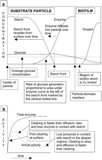
In mechanistic descriptions of the effect of nutrient concentrations on growth in SSF, it is not valid to relate the specific growth rate with the nutrient concentrations obtained by mashing the substrate particles prior to analysis. The mass transfer limitations within SSF particles cause concentration gradients of nutrients to arise and therefore the actual nutrient concentrations experienced by the organism are not equal to the average concentrations given by the mashing procedure (Fig. 4) [83–85]. In fact, microbial cells or hyphal tips

Fig. 4. a The concentration gradients which arise within substrate particles, shown for the growth of an amylolytic unicellular organism on a substrate containing starch. b The consequences that clearing of starch at the particle surface has on the rate of glucose generation within the substrate particle by the glucoamylase

located in different regions of the particle will be experiencing different nutrient concentrations. Likewise, there are oxygen concentration gradients within the substrate and cells or hyphal tips located in different regions of the particle will be experiencing different oxygen concentrations [86].

It is logical to express the specific growth rate of a cell or a hyphal tip at a particular location in the same manner that is common in SLF, namely by use

of the Monod equation. For example, the effect of oxygen on the growth of aerobic microorganisms can be described by a Monod relationship [87]:

KO2 + CO2ΩZ

where the notation ΩZ signifies that the value is for a particular location in space. The subscript O2 signifies that this is the effect of oxygen on the specific growth rate. Other subscripts are used below to distinguish the effects of other environmental variables. The Monod equation can also be used to describe the effect on the specific growth rate of glucose as the sole limiting nutrient [84, 85]:

If the substrate is inhibitory at high concentrations then a substrate inhibition term can be included:

Although the last equation is presented here in terms of local nutrient concentrations, in the work in which it was used it was based on the average substrate concentration [88]. In this case the relationship between specific growth rate and nutrient concentration is purely empirical: it can only be determined from experiments done with the particular system modeled, and parameters are likely to change with small changes in the system, such as particle size. In contrast, the mathematical models in which Eqs. (2) and (3) were used included expressions describing the diffusion of glucose or oxygen or both. In this case the parameters of the equation can be determined in an independent system, such as liquid culture, in order to remove mass transfer limitations. Changes in system behavior due to changes in particle size would be taken into account by the diffusion equations, and there would be no need to adjust the parameters of the expression for the specific growth rate.

Models of bioreactor performance usually only take into account the intraparticle diffusion of nutrients if heterogeneity at the macroscale across the bioreactor can be ignored [89, 90]. For bioreactors in which there is heterogeneity at the macroscale, and even in some cases where there is no macroscale heterogeneity, to simplify the model it is common to use empirical equations that do not rely on nutrient or oxygen concentrations. These empirical approaches are commonly based on the logistic equation, which reasonably describes the biomass profiles found in many SSF systems, with extended periods of acceleration and deceleration of growth:

with X corresponding to the biomass concentration (in kg-biomass kg- substrate–1).

The deceleration of growth as X approaches Xmax could be due to nutrient limitations, accumulation of inhibitory products, or maximum packing densities based on steric limitations [91] although in practice the value of Xmax is usually simply taken directly from experimental biomass profiles. Note that mmax is also typically determined empirically. However, with the assumption that each fungal hypha branches to give identical daughter hyphae which extend at the same rate as the mother hypha, these macroscopic parameters can be related to microscopic parameters such as hyphal branching frequencies and hyphal extension rates [92, 93].

Linear and exponential kinetics can also apply for a significant part of the growth phase. During an exponential growth phase m remains at mmax , whereas during a linear growth phase the growth rate itself is a constant. In this case there is a need to impose an external condition to prevent predictions of infinite growth; for example, that the growth rate equals zero when the biomass concentration reaches a particular value. In any case, linear or exponential growth profiles rarely persist for the whole of the fermentation time, and it may be necessary to divide the fermentation time into different phases. For example, to describe a fungal growth profile with early exponential growth followed by an extended period during which the growth rates slowly decelerates, the following

At time ta there is a switch to deceleration phase kinetics, described by

dX

5= mmax L · e–k (t – ta ) (7)

dt

where the factor L describes an instantaneous decrease in the number of actively extending hyphal tips as the fungus enters the deceleration phase. During the deceleration phase there is a further first-order decay in the number of actively extending hyphal tips, with first order rate constant k.

The appropriate form of an empirical equation can only be decided after the collection of experimental data. This should be done with small substrate masses so that interparticle heat and mass transfer processes are not limiting. The integrated form of the growth equation can be fitted against the biomass fermentation profile by linear or non-linear regression to extract the parameter values. In doing this, it must be clear whether the biomass is expressed in absolute concentration terms (i.e., kg-biomass m–3) or as in relative concentration terms (i.e., kg-biomass kg-dry-matter–1). Since the amount of dry matter decreases during the fermentation due to the loss of carbon in the form of CO2 , these two expressions cannot simply be converted from one to the other by multiplying by a constant [95].

4.1.2

Effect of Temperature on Growth

Temperature is an important variable in SSF systems because the difficulty of removing waste metabolic heat from the substrate bed means that the temperature rises within the substrate bed, with the problem becoming more severe as the size of the substrate bed increases. As a result, in most large-scale bioreactors the microorganism at any location within the bed is subjected to a temporal variation in temperature, with the degree of variation depending on the effectiveness of cooling at that location in the bed. Usually there is an initial period of growth at the optimum temperature for growth, during the early period when the biomass density is low and therefore the rate of release of waste metabolic heat is low. However, as the biomass concentration increases the growth rate increases and therefore the rate of heat production increases. If the heat production rate exceeds the heat removal rate at that location in the bed, then the temperature increases. In poorly cooled regions of the bed, temperatures close to the maximum temperature for growth may be reached, with this temperature being maintained for periods as low as 1 h to as long as 50 h. Later, growth decelerates, possibly due to negative effects of the high temperature, but also possibly due to steric limitations on biomass density or nutrient exhaustion, and, as a result of the decreased heat production rate, the temperature falls again. As a result of the inevitability of temperature rises in almost all types of bioreactors, it is essential to incorporate a description of temperature effects on the growth kinetics.

To date, studies aimed at describing the effect of temperature on growth kinetics have obtained data using an experimental procedure which can be referred to as the “isothermal approach”: a range of cultures are incubated at a range of temperatures, with each culture being maintained at a constant temperature throughout the fermentation. This can be achieved by using a small enough substrate sample (several grams) so that heat removal limitations are negligible. The specific growth rates are then plotted as a function of the incubation temperature and a mathematical expression, usually an Arrheniustype expression but sometimes simply a quadratic fit, is fitted to the data. In those cases where temperature-related death of the biomass is not taken into account the expression describes the net growth rate and needs to be able to describe the decrease in growth rate above and below the optimum temperature for growth. Empirical expressions include the double Arrenhius expression [96]:

1 + B. exp 004 R(T + 273.16)

where temperature is in °C. Alternatively, simple polynomial equations can be used [87, 97, 98]. The effect of temperature on the parameter Xmax in Eq. (5) can also be described if data for this parameter is collected during the experiments. Typically this can be fitted with a quadratic function [96].

It is also possible to divide the biomass into living and dead biomass and to include equations for temperature-related death. Arrhenius-type relationships can be used to describe the effect of temperature on both the specific growth rate and the specific death rate, giving a net growth rate [99]:

In this case both of the rates increase with temperature, but the death rate is negligible below the optimal temperature. Above the optimal temperature the death term increases faster than the growth term, so the net specific growth rate falls. In this case the equation was fitted to data collected using the isothermal approach using non-linear regression.

A slightly different approach was taken by Smits et al. [100]. Rather than describing the death of biomass itself, they incorporated an inactivation term into their equation relating oxygen uptake to growth. This corresponds to a decrease in specific respiration activity as a result of aging processes. The inactivation term was expressed as an Arrhenius function of temperature:

where md0 is the basal specific inactivation rate.

As mentioned above, to date the effect of temperature on growth and death kinetics has been based on data obtained using the isothermal method. However, recent work indicates that the growth and death kinetics of a microorganism which starts growing at the optimum temperature for growth and is later subjected to a rise in temperature is not adequately described by the equations obtained using this isothermal approach. In the bioreactor model of Saucedo-Casteneda et al. [96], the model could not describe the experimental temporal temperature profiles if the specific growth rate was allowed to decrease as the temperature rose above the optimum temperature according to the expression obtained from isothermal approach data. Good agreement with the experimental results could only be obtained if the growth rate was assumed to remain constant as the temperature increased. Ikasari et al. [101] mimicked the temporal temperature profile in SSF of Rhizopus oligosporus by making a step upshift in temperature from 37 °C to 50 °C after 20 h of fermentation and a downshift back to 37 °C 10 h later. Growth rates close to the growth rate before the temperature upshift were maintained for several hours at the higher temperature. Furthermore, the upshift had delayed deleterious effects which were not reversed by returning the culture to 37 °C. More work needs to be done with a wider range of organisms and various temporal temperature profiles to obtain sufficient kinetic data to allow the effect of a varying temperature on growth to be modeled adequately.

4.1.3

Effect of pH on Growth

Microbial growth is usually significantly affected by the local pH. This has important consequences for SSF processes since pH gradients arise within the substrate particles, and although pH correcting solutions can be added to the substrate in mist form with some bioreactor designs, fine pH control in SSF is impracticable [84]. Models have been proposed which relate growth rate to pH based on empirical equations describing experimental data for the effect of pH on growth rate [102, 103]. However, the diffusion of protons within the substrate particles was not included in the equations, which raises questions as to the validity of such models, since the microbial growth response will depend on local pH and not some global average.

4.1.4

Effect of Water Activity on Growth

Relatively little effort has been made to incorporate the effects of water activity within bioreactor models, and it is done by using empirical expressions to obtain an expression for mw . Pitt [102] assumed that the specific growth rate fell linearly between an aw of 1 and the minimum aw for growth while Muck et al. [103] broke the curve into several linear segments. Data for the effect of water activity on the growth of fungi is commonly obtained by measuring the effect on the radial extension rate of colonies. Assuming that the width of the peripheral growth zone of the colonies is constant despite variations in water activity, then the radial extension rate will be directly proportional to the specific growth rate [104], and therefore such data can be adapted for SSF.

In colony extension rate data there is typically an optimum water activity at a value somewhat less than aw =1, with the radial extension rate falling off exponentially as the water activity decreases below this optimum [105, 106]. The following equation describes the exponential part of the curve:

aw

r = A ln 51+ rm (11) aw0

where A is a constant, and rm is the radial extension rate at the optimal water activity for growth, aw0 .

4.1.5

Combining Environmental Effects

The simultaneous variation of various environmental variables within SSF systems raises the question of how their effects on growth should be combined. The best idea is to identify a value for mmax , the specific growth rate at the optimum combination of T, pH, water activity, and with saturating nutrient concentrations. The relative effects of the different environmental variables can

whole surface covered, further increases in density occur by growth above and below the surface.

The biomass in SSF is distributed spatially in one of two forms. Unicellular organisms such as bacteria and yeasts grow as a moist film on the surface of the substrate particle. This film will have a constant biomass density, and the intercellular spaces will be occupied by moisture. Mycelial organisms such as fungi and streptomycetes may extend above and below the substrate surface. Steric limitations associated with branching frequency and branch angles prevent high packing densities. Maximum packing densities can be 15–34% of available volume [91, 108]. In unmixed fungal SSF processes, within the substrate particle and within thin moisture films at the substrate particle surface, the spaces between hyphae will be occupied by an aqueous phase. However, the hyphae extending above the surface will typically be in direct contact with air [109]. In processes with mixing, the mixing action tends to squash the fungal mycelium to make a moist film at the surface, which will behave similarly to a biofilm of unicellular microorganisms [110].

Penetration into substrates is an important phenomenon which has been observed experimentally but has not yet received modeling attention. Ito et al. [111] showed that the concentration of penetrative hyphae decreased exponentially with depth in rice koji. Depths of penetration by hyphae of Rhizopus oligosporus into soybeans during the production of tempe vary from 0.4 mm to 2 mm, with the majority of penetrative hyphae extending to depths of 0.4–0.7 mm [112, 113]. The average frequency of penetration into the soybean was one penetration per 785 mm2 of surface area. The majority of penetrations occurred in the intercellular spaces during growth on soybean cotyledons. Penetration into substrates where the cellular structure had been disrupted was easier. In soybean flour, R. oligosporus penetrated to depths of 0.5–1 mm, with a maximum depth of penetration of 5–7 mm [113].

Penetrative hyphae can potentially play an important role in making the substrate accessible to enzymes [113]. On the basis of expected molecular diffusion coefficients of proteins in solutions of 10–11 m2 s–1, enzymes would be expected to diffuse to depths of about 1 mm after 40 h, or even less if lower effective diffusion coefficients of around 10–12 m2 s–1 occurred, such as might be expected within solid substrates [113]. Therefore enzyme diffusion occurs at a rate similar to hyphal penetration rates. As a result, the contribution of hyphal movement and release of enzyme from the hyphal tip would be significant in allowing the enzyme to reach greater depths than if the enzyme was simply released from the surface. Note that in modeling work to date enzyme release has been assumed to occur only at the interface between the substrate and biomass phases [84, 85, 114].

Early modeling studies of growth ignored the microbial growth form, simply expressing it as a concentration per area of substrate surface [83, 84]. Effectively these models assume that glucose crossing the surface is converted instantaneously into biomass. There is no diffusion of glucose in the biomass layer. Most of the more recent models have modeled growth in the form of biofilms, assuming a phase of constant density which increases in height during growth [85, 114, 115], and in which the value for oxygen diffusivity is that for