New Products and New Areas of Bioprocess Engineering

Fig. 4. Multistage electromagnetic separator compared with a magnetic chromatography column

ficient that can be predetermined. By determining a specific set of conditions (i.e., constant geometry, magnetic field, materials, etc.), the selected volumetric susceptibility range becomes a function of the time that the particles are in motion. The relationship between the susceptibility range separated and time could then be condensed into a single mathematical equation. The constant produced as a result of the fixed variables would give an indication of the ratio of particles in the upper cavity compared with the number of particles in the lower cavity at the separating time.

Experiments using inactivated magnetotactic bacteria and a single permanent magnet repeatedly confirmed that rather weak magnetic particles could be translated at a controlled velocity through an aqueous medium over distances up to 2 cm.

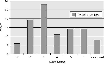
A magnetically adapted ADSEP was used to reduce the above principle to practice. Using large (1–2-mm) paramagnetic beads from Polysciences, Inc. (Warrington, PA, cat. no. 19131), a series of cylindrical magnets of increasing strength with increasing cavity number was positioned above six consecutive cavities of the ADSEP upper plate in the programmable ADSEP base device. These commercial particles have a broad distribution in size and susceptibility (shown in Fig. 5). The permanent-magnet pole pieces were of the same diameter as the cavities. In the example described below, particles were magnetically attracted to the upper cavity, without agitation, during 5-min intervals of exposure to successively increasing magnetic fields. The number of particles captured in each upper cavity was then counted using a microscope and hemacytometer. The results at various field strengths and gradients are given in Table 1.

Fig. 5. Histogram of particles separated in each stage of MAGSEP using increasing fields and gradients, and Dt = 5 min

Table 1. Particle separation test data for MAGSEP

The effect of adjusting exposure time was explored, and it was found that short exposures result in less particle capture at early stages and aggregation by stronger magnets at later stages. This important discovery that proper temporal programming can prevent aggregation makes the MAGSEP concept feasible. In addition, the magnets used in the above experiment had pole fluxes ranging over two orders of magnitude, and the weak magnets were shown to attract large beads while, in separate experiments, the strong magnets were shown to attract weak particles such as magnetotactic bacteria (data not shown).

2.1.3

Theory and Mathematical Models

The range of magnetic field required for cell separation is obviously decided by the magnetic and mechanical properties of the cells. A review of the mathematical formulae that are relevant to cell extraction and their illustration by selected examples was presented well by Zborowski [43].

The magnetic field is a space domain where an electrical charge ‘e’ moving with velocity ‘ve’ experiences a magnetic force ‘Fm’, given by

where ‘I’ is the current intensity, l is length of element, and B is the magnetic field intensity (kg A–1 s–2 or Tesla, T ) given as

where mo is magnetic permeability of free space and H is the magnetic field strength (A m–1). The presence of matter in the magnetic field modifies the field fluxes at given constant field strengths. The magnetic properties of matter are defined by induced polarization M to account for the variation in magnetic flux. For isotropic media

where cm is magnetic susceptibility. In the uniform magnetic field the magnetic particle undergoes rotation until Maxwell stress tensor becomes zero and then remains stationary with respect to the medium. In the non-uniform field, differences in the Maxwell stresses result in a net force Fm acting on the magnetic particle given as

where Vp is the volume of the particle. In the simplest one-dimensional case, using Eq. (3), it can be written as

dB

Fm = Vp cm H 41 (5) dz

In homogenous media, magnetic field B is parallel and proportional to the magnetic field strength H. Magnetic force lines are defined as curves which are

tangent to the direction of vector Fm . In general, due to non-linear relationship between the magnetic force Fm and the magnetic field H, the lines of magnetic force do not follow the lines of magnetic field B. In other words, even in homogenous media, the lines of magnetic field do not represent the lines of force exerted on the elementary dipole. The correct representation of such forces are the lines of the magnetic force Fm . This is drastically different from the static electric field, in which electric force lines are synonymous with electric field lines.

Now the work required to bring all the components of the magnetic system from infinity to their given spatial position is defined as magnetostatic potential energy Um , which with the help of Eqs. (2) and (3) can be given as

Vp cm B2

Um = Vp cm um = – 03m (6) 2 o

where um is magnetic energy density, given by –B2/2m0 . The relationship between the force and the potential energy leads to the following expression of the magnetic force:

Vp cm—B2

Fm = –—Um = –Vp cm—um = 05m (7) 2 o

The direction of the magnetic force Fm relative to the energy density gradient

—B2 depends on the sign of cm . For paramagnetic substances, cm > 0 and the force vector points toward the direction of the maximum increase in magnetic field energy density, termed magnetic attraction. For diamagnetic substances cm< 0 and the force vector points in the opposite direction to the maximum increase in the field energy density, termed magnetic repulsion. When the particles are suspended in a medium of magnetic susceptibility cm , then in the above expression cm is to be replaced by Dcm . Consequently the above discussion applies to Dcm rather than cm .

Thus the very basis for all magnetic cell extractors is the observation that forces acting on small magnetic particles follow the lines of gradient of the magnetic field energy density.

2.1.3.1

Model for Viscous Medium

A simple mathematical model is developed based on the theory discussed, till now, for the motion of magnetically labeled cells in a viscous medium in the presence of magnetic field [43]. The following assumptions are involved:

1.Cells are small compared to the characteristic magnetic field and fluid flow dimension

2.Cells are treated as magnetized rigid spheres while calculating magnetic and fluid drag forces

3.Specific density of the cell is similar to that of the medium

4.Inertial forces are too small to be considered when compared with the viscous ones

By taking the dot product of the magnetic field and the gradient of the magnetic field, the following differential relationship is determined:

This relationship, combined with the above assumptions to simplify the magnetic force equation, yields the scalar magnetic force relationship similar to that given in Eq. (9). If all variable parameters for the MAGSEP experiment in this equation (B and particle size ap) are set, then the susceptibility difference, Dcm is the controlling variable governing the magnetic force. Based on this calculation, the separation of the cells as it relates to the susceptibility difference can be governed by controlling the magnetic field B, the vertical height of separation Dz, and the time interval required for separation, Dt.

The volumetric susceptibility difference Dcm can be measured by sampling a distribution of particle positions (which is a function of their velocities). If the particles are placed in a thin flat layer across the bottom of a cavity and covered with a solution to a depth Dz, the particles can then be aligned below a shallow upper cavity with an activated magnet. The magnetic field of the upper magnet can then attract particles for a time Dt, and when a sufficient amount of particles have migrated into the shallow upper cavity, the cavities can be halfstepped to separate the particles as shown in Fig. 3. The volumetric susceptibility can then be calculated by the following relationship:

B · 41 dz

where vp is the velocity, and can be assumed to be equal to Dz/Dt. The number of particles transferred represents a distribution of the total particles and is also a representation of the number of particles within a volumetric susceptibility range. If enough separation in these stages takes place, then this volumetric susceptibility range can be assumed to be an absolute volumetric susceptibility. Further modeling of magnetic extraction in MAGSEP is in progress.

Continuous flow magnetic cell sorting using soluble immunomagnetic label and the corresponding theory was presented by Zborowski et al. [44].

2.2

Electrophoretic Extraction

2.2.1

Existing Methods – Brief Analysis

Electrophoresis is a leading method for resolving mixtures of charged macromolecules (either proteins or nucleic acids) or cells. The electrophoretic separation of proteins without gels has been a long-standing goal of separation research [45, 46]. Electrophoretic separations are influenced by many factors including the size (or molecular weight), shape, secondary structure, and charge of the macromolecule or cell. These features can influence electrophoretic properties either separately or jointly. In order to achieve the required scale-up scientists and engineers resort to flowing methods [46–48]. Scale-up of electrophoresis is hindered by ohmic heating. The heat generated is equal to the product of the current and voltage, and this heat can cause free convection and mixing within the system. Too much heat can also denature the labile biomolecules or cells.

Decades of research in free electrophoresis have identified thermal convection [49], electro-osmosis [50], particle sedimentation [51], droplet sedimentation [52], particle aggregation [53], and electro-hydrodynamic zone distortion [54] as the major obstacles to scale-up. Free electrophoresis has not gained popularity as a preparative or industrial separation method owing to these gravity-dependent characteristics. Density gradients [52, 55] or elaborate flowing devices have been required up to now to stabilize free fluid systems and/or the particles suspended in them while they are non-isothermally heated by the passage of an electric current. Without the need to prepare density gradients and/or use elaborate flowing systems, free electrophoresis could enjoy more widespread use, because it is a high-resolution separation method that does not require adsorption to solid media and the subsequent solids handling. Furthermore, it can handle particles (cells) as well as solutes (macromolecules) alike. To name a few, specific applications of free electrophoresis include the separation of different cells of peripheral blood and bone marrow in hematological and immunological research and potentially in clinical therapeutic applications [56], and the separation of proteins from body fluids, tissue extracts, and fermentation broths in biotechnology [57].

None of these principal gravity-dependent and gravity-independent processes have been investigated in multistage electrophoresis, which is designed to minimize the impact of these processes on separation quality. All of these processes have been studied in the past in applications to other forms of free electrophoresis as reviewed by Todd [34, 41].

Thermal convection, which in turn causes mixing, is induced by ohmic heating when current passes through the buffer and heats the buffer non-uni- formly [49]. Above a critical Rayleigh number (Rac ), convective circulation sets in, and it occurs in both static and flowing electrophoresis systems [54, 58]. The Rac is unexpectedly low in certain flowing electrophoresis applications, so that thermal convection is a significant deterrent to the development of electro-

phoresis as an industrial separation tool [59]. Under most circumstances in particle separations, conditions can be arranged so that the sedimentation of individual particles, say cells, can be minimized, but not always [51]. Finally, the diffusion-driven formation of droplets containing high concentrations of particles or solutes [60] results in ‘droplet sedimentation’, and at very high concentrations of particles in density-gradient electrophoresis [52] but not in low-gravity electrophoresis [54].

Another type of mixing problem encountered in free electrophoresis, although less critical compared to ohmic heating, is the mixing caused by gas release at the electrodes. This problem is addressed by employing non-gassing electrodes [61] or membrane-separated electrodes [62]. This experience points to the possibility of using non-gassing Pd electrodes (as in the present work) rather than the more complicated membrane based system of Tulp et al. [63].

A score of methods has been developed to effect free electrophoresis [41]. These methods can be broadly divided into static and flowing methods, neither of which has satisfactory capacity for application as a manufacturing tool. Batch and continuous methods have also been developed. In almost all cases maximum sample input rates have been of the order of a few milliliters per hour. In one important case, Tulp et al. [63] designed a re-orienting free electrophoresis device consisting of a flat disk-shaped container with thin sample bands and a short migration distance. The top and bottom electrode fluids served as coolant, the total height of the separation column was 1–2 cm, and its diameter was greater than 15 cm. The distance between unrelated separands was about 1–2 mm, and this distance was increased during fractionation after electrophoresis by re-orienting the disk.

Based on research experience and needs identified for free electrophoresis in various fields of bioprocessing and analysis such as virology, endocrinology, enzymology, hematology, and mammalian cell culture [64–69], in the present study an attempt is made to overcome the major bottlenecks of free electrophoresis.

2.2.2

Multistage Electrophoretic Method

The multistage electrophoretic method has been developed by combining free electrophoresis and multistage extraction and is explored as an improved alternate method for the purification and concentration of cells or macromolecules. The present discussion is restricted to cells and particles. The present design is based on a derivative of the thin-layer multistage extractor design of Albertsson [70] and Treffrey et al. [71] and called ADvanced SEParation apparatus (ADSEP), designed by SHOT, Inc. [42].

To test this method extraction of fixed human red blood cells and latex suspended in 0.01 mol l–1 phosphate buffer was performed at different electric field strengths such as 0.05 V m–1 or 0.1V m–1. A simple mathematical model was developed (discussed in Sect. 2.2.3) to describe the mass and heat transfer during the electrophoretic separation process in the countercurrent extractor employed. The experimental results agree reasonably well with those predicted

by the model, which suitably predicts separations of mixtures of cells or molecules having different electrophoretic mobilities as well.

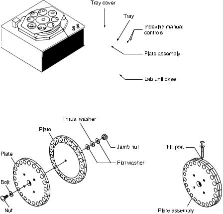
The latest version of the ADSEP fabricated in collaboration with SHOT, Inc [42] is described in detail in Figs. 6 and 7. The extractor consists of a 22-cavity multi-stage thin layer extraction system [71]. Half-cavities oppose each other in disks that are sealed together and rotate with respect to each other. The half cavities are disk shaped, and top cavities have flat tops while bottom cavities have flat bottoms. Both contain palladium (Pd) metal electrodes that produce an electric field when the two cavities are in phase with each other. This extractor, like the Tulp device [63], takes advantage of short column height to maintain isothermal conditions. Each cavity is only a few mm in height so that the fluid within it remains isothermal during the application of an electric field that transfers the separand particles or molecules from the bottom to the top cavity. As each separand is transferred to a new cavity, it is either drawn into the upper cavity by the electric field or left in the lower cavity, depending on its

Fig. 6. ADvanced SEParation (ADSEP) apparatus

Fig. 7 a, b. Assembly of multistage extraction plates containing the chambers: a plates; b filling ports

160 K.S.M.S. Raghavarao et al.

electrophoretic mobility. The assembly of the plates containing the chambers is shown in Fig. 7a. Identically designed plates assure uniform loading and sealing when the plates are clamped together. The experimental samples are loaded and withdrawn through the fill ports located on the side of each plate as shown in Fig. 7b. ADSEP is driven by an independent power supply (Lamda, Model No. LP-532-FM) for rotating the plates to bring the chambers into interfacial contact with each other. This ADSEP was modified to use as ELECSEP by replacing the chamber bottoms with metal cover plates. Electrodes are kept over these cover plates with gaskets in between them.

Preliminary electrophoretic transfer experiments were carried out [72] with two types of particles, fixed human red blood cells and latex particles (average diameter is 3.5 mm and 2.3 mm, respectively). The particles were counted by hemacytameter with a minimum of three counts per fraction. Average values of duplicate experiments were reported.

Fixed human red blood cells, in the concentration range of 90 – 245 ¥ 104 ml–1, were placed in suspension in 0.01 mol l–1 phosphate buffer (pH 8.0) in the lower cavity of stage 1 in a total volume of about 0.4 ml. A field of known intensity (0.05 Vm–1 or 0.01Vm–1) was applied for a specified time period (30 s or 60 s) then a fresh top chamber containing buffer only was aligned with the bottom chamber of stage 1. This process was repeated until several transfers had been completed. Cells were then removed from the top cavities, and the fraction of the original population transferred at each step was obtained by counting the suspended cells with a hemacytameter.

Precautions are required when using sliding chambers. Swapping of the liquids between the chamber liquid surfaces occurs during the time period while the chambers approach each other for the extraction transfer step and depart after the transfer. The swapping of liquid and enhanced mass transfer associated with such hydrodynamic flow for similar equipment was reported [73]. The schematic diagram indicating the swapping of liquid and flow pattern during the alignment and separation of the chamber is shown in Fig. 8 [73]. In order to assess the magnitude of cell migration due to this phenomenon, a few control experiments were performed without the application of an electric field. Results are shown in Table 2.

Considerable numbers of cells are transferred due to the hydrodynamic flow during transfer steps, especially in the initial steps. This problem is alleviated by giving sufficient settling time for the cells to settle toward the bottom of the lower cavity and by considerably reducing the speed at which the cavities are aligned during the transfer steps.

Table 2. CCD without application of electric field