Friesner R.A. (ed.) - Advances in chemical physics, computational methods for protein folding (2002)(en)

correlated with others (Table IV), consideration of all of them is useful because exhaustive enumeration or a genetic algorithm (GA) is employed to determine which to include for optimal fitting and prediction.

The database consists of 33 proteins. Twenty-four of these fall into six structurally related groups, and nine are structurally unique. The former are SH3 domains [1NYF (82 to 148), 1PKS, 1SHG, and 1SRL], Ig-like b-sandwiches [1FNF (1326 to 1415), 1FNF (1416 to 1509), 1HNG, 1TEN (802 to 891), 1TIT, and 1WIT], members of the acylphosphatase family (1APS, 1HDN, 1PBA, 1URN, and 2HQI), cytochromes (1HRC, 1HRC-oxidized, 1YCC), cold shock proteins [1CSP and 1MJC (2 to 70)], l-repressor variants (1LMB wild type and G46A/G48A), and ubiquitin variants (1UBQ wild type and V26A). The remainder of the proteins are 1COA (20 to 83), 1DIV (1 to 56), 1FKB, 1IMQ, 2ABD, 2AIT, 2PDD, 2PTL (94 to 155), and 2VIK. Numbers in parentheses indicate the residue numbers of the domain or fragment studied.

To cross-validate the results, each group of structurally related proteins is left out of the training set in turn and used to test the network. Such a partitioning scheme (in contrast to a jackknife one, for example) minimizes the likelihood of biasing the results in favor of structural descriptors (see Section II). Its use yields true predictions (denoted ‘‘cv’’) in contrast to fits of the data, in which all the proteins are included during the training (denoted ‘‘trn’’). The latter tend to yield inflated accuracy statistics, but we describe them here as well for comparison with earlier studies [12,13,20,47], which failed to cross-validate their results [however, it should be noted that the relationship in Ref. 12 has been used successfully for blind predictions (K. W. Plaxco and D. Baker, personal communication)].

C.Single-Descriptor Models

We begin by examining the relationship between log kf and each individual descriptor.

1.Linear Correlations

The first column of statistics given in Table I contains the Pearson linear correlation coefficients between the descriptor values (x) and log kf ðrx;log kf Þ. This is the statistical measure used by Plaxco et al. in their analysis of a subset of the descriptors considered here [12,14]. Consistent with their results, the two coefficients with the largest magnitudes are associated with the contact order (c and c=n). Several descriptors not examined by Plaxco et al. [12,14] exhibit jrx;log kf j > 0:5 as well: the a-helix content and propensity (h and ph), total helix content (a), and b-sheet content (e). Additional linear statistics are provided in Table V. Physical interpretations of the results are given in Section IV.E.

2.Neural Network Predictions

The second and third columns of statistics in Table I measure the ability of a single-input neural network to predict the folding rate. They contain Pearson

linear correlation coefficients (rtrn and rcv) between observed and calculated values of log kf ; thus, only positive values of r are significant. Because there are only 24 different input possibilities, it is feasible to consider each one in turn, so that use of a genetic algorithm is not necessary at this stage. However, the NN weights depend on the random number generator seed through the training procedure. Consequently, for each descriptor, the network was trained independently with ten different seeds. The maximum correlation coefficient for each set of 10 networks corresponding to a particular descriptor is listed in Table I; the average standard deviation for a given descriptor was 0.03 for rtrn and 0.06 for rcv.

As stated above, the coefficients denoted ‘‘trn’’ are for results obtained with networks trained on all 33 proteins; in other words, they are not true predictions since all the data are included in the training set. For descriptors that are linearly related to log kf ; rtrn is expected to be comparable in magnitude to rx;log kf (in fact, for linear regression, rtrn ¼ jrx;log kf j), whereas, for ones that are non-linearly related, it should be higher. Thus, rtrn can be viewed as essentially a nonlinear version of the statistic employed in Ref. 12. Accordingly, most of the descriptors that exhibit high rtrn were included in the analysis of rx;log kf .

The coefficients denoted ‘‘cv’’ are for the predictions obtained with the structurally based cross-validation scheme. Negative values of rcv indicate that the accuracy of the network is lower than that which would be obtained from random guesses. If a network fails in this way when confronted with novel test data, it has derived a spurious relationship by memorizing the information in the training set at the expense of learning more general rules. The highest rcv do correspond to the highest rtrn, but overall the cross-validated coefficients are much lower. The large differences between rtrn and rcv in many cases (Table I) make clear that the former is a relatively indiscriminate statistic for such a small database. If linear regression is used, rtrn and rcv are often closer due to the decreased flexibility of the fitting method (Table V). However, such an approach fails to identify nonlinear relationships and can hide complexities in the results.

In summary, the contact order yields relatively good prediction of log kf but is not alone in doing so. Several measures of the propensity of the sequence for a given structure also exhibit significant relationships with the folding rate. Although rcv values for the various descriptors obtained from the secondary structure prediction program (indices 16 to 21 in Table I) are lower than those for measures of the known native structure (indices 6 to 15), the former correlations may be sufficiently high that the calculated descriptors could be used to identify particularly fast or slow proteins without the need for highresolution structures. The stability, which has been suggested to be of importance based on model studies, exhibits no clear relation to the folding rate. An essential additional point of the single-descriptor analysis is that large differences are observed between most of the values obtained with and without cross-validation. This highlights the need for care in assessing the significance of correlations when working with small numbers of sequences.

D. Multiple-Descriptor Models

We present results for twoand three-descriptor models; addition of a fourth descriptor yielded no significant improvement in predictive accuracy. In the twodescriptor case there are only 276 possible input combinations, so we examine each explicitly, whereas, in the three-descriptor case there are 2024, so we use the genetic algorithm (GA) to optimize the descriptor selection. Use of the GA in the two-descriptor case gives models of comparable quality to the exhaustive search, but this test of the algorithm is not very stringent because the space of input combinations is small. Because both the GA and the NN depend on the random number generator seed, several trials were performed in each case (as detailed in Section IV.D.2).

1.Two Descriptors

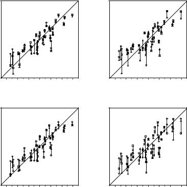
The best five two-descriptor models are shown in Table VI, and selected examples to illustrate the types of behavior that are observed are shown in Fig. 2.

The Best (as Measured by rcv) Five Two-Descriptor Models Obtained by Examining All Possible Combinations for Ten Different Random Number Generator Seedsa

aFor the calculation of E, q2cv was compared with that for c=n. Statistics for linear regression and additional measures of the predictive accuracy are available in Tables VII and VIII.

rcv values are close to that for c=n by itself (Table I); the NN ignores the randomized descriptor. The fact that the rcv values for the actual data are two to four standard deviations above the average rcv values for the randomized data demonstrates that the improvement is significant and is not due to the increase in the number of fitting parameters.

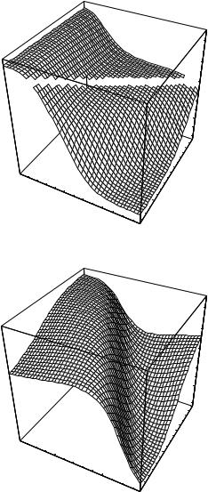
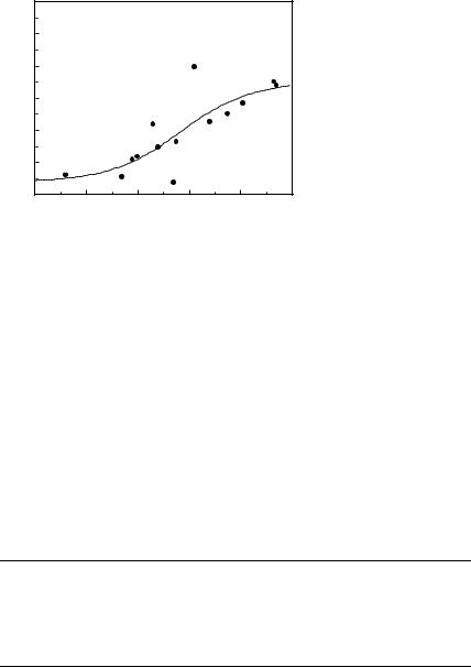
The best predictions are obtained with G=n paired with c=n ( G with c is the sixth best set of inputs with rcv ¼ 0.77 and E ¼ 0.76) This combination of input descriptors was investigated previously [15], but it is of interest that it ranks first in the exhaustive search performed here. To better understand the physical basis for the correlations, we show the dependence of log kf on c=n andG=n in Fig. 3a. When c=n is small (c=n 19; mainly a-helical proteins), folding is always fast (kf > 400 s 1), whereas when c=n is large (c=n 25; either mixed-a/b or b-sheet proteins), the rate spans over three orders of magnitude. Thus, proteins with lower contact orders fold fast regardless of their stabilities, whereas for those with higher contact orders, the rate increases with G=n. As described in Ref. 15, a single-input neural network can be trained to predict log kf from G for the 14 proteins with c > 21 (Fig. 4); rtrn ¼ 0:81, and rcv ¼ 0:64, which confirms that stability plays a significant role in determining the folding rates of mixed-a/b and b-sheet proteins. For these 14

TABLE VII

Randomization Tests for the Models in Table VIa

aIn each case, the second descriptor listed was shuffled 10 times, and the networks were trained as for the original data. Values shown are averages for the 10 trials; ranges indicate standard deviations.

¼ 0:23.

Two of the other models in Table VI combine the contact order with a measure of the a-helical propensity: c=n with either Ph or ph: These pairings essentially reflect the results of the previous section. The remaining model couples c=n with nc, which reveals a secondary dependence on protein size. Consistent with the sign of rnc;log kf (Table I), the functional dependences of log kf on these descriptors for the models in Table VI indicate that shorter proteins fold faster than longer ones (Fig. 3b).

2.Three Descriptors

As mentioned above, there are 2024 possible combinations of three descriptors, so we use a GA to identify the inputs that are likely to yield the greatest predictive accuracy. Use of the GA requires selection of a particular measure of predictive accuracy to decide which models to keep at each cycle. Because we are interested primarily in cross-validated predictions, rcv is a natural choice. However, the structurally based partitioning scheme is less straightforward to automate than a jackknife one. Consequently, for the GNN, we used the Pearson linear correlation coefficient for the jackknife cross-validated outputs (rjck) and subsequently tested each selected combination of descriptors with the structurally based cross-validation scheme (rcv). We performed five GNN trials, from each of which we saved the best 20 models. Of these 100 models, 46 were unique, and each of these was subjected to 10 trials with the structurally based cross-validation scheme.

In general, the GA combines the descriptors that were identified above by the two-dimensional exhaustive search (c; c=n; G; G=n; and nc) to further refine the predictions (Tables IX to XI and Fig. 2). The propensity for sheet structure ðpeÞ appears in two of the five models; not surprisingly, it is strongly anticorrelated with the propensity for helical structure, which appeared in Table VI

¼ 0:89). In considering these results, it is necessary to keep in mind that the database is small, so that there is a danger of overfitting (but see Table X). Nevertheless, given this disclaimer, we see that simultaneous consideration of multiple descriptors improves prediction of the folding rate and that both the

size and the stability play significant secondary roles that could not have been anticipated from the single-descriptor analyses.

E.Physical Bases of the Observed Correlations

Consistent with earlier, single-descriptor linear analyses of protein folding [12,13,50], the primary determinants of the folding rate are measures that characterize the native structure; that is, proteins with more sequentially local interactions tend to fold faster. As discussed below, the equilibrium structure and the kinetics are connected by the fact that the structure of the transition state resembles that of the native state in many small proteins [50]. Thus, the kinetics and the underlying thermodynamics of the reaction are affected in a similar way, in accord with linear free energy relations.

The microscopic origin for the statistical dependence of the folding kinetics on the structure is the stochastic diffusive search that is required to find the

TABLE IX

The Best (as Measured by rcv) Five Unique Three-Descriptor Models Obtained from the GNN Protocol for Ten Different Random Number Generator Seedsa

aFor the calculation of E, q2cv was compared with the highest observed q2cv of the six possible twodescriptor models that could be formed from the three selected inputs (corresponding to the unshuffled pair in Table X). Statistics for linear regression and additional measures of the predictive accuracy are available in Table X and XI.