

Friesner R.A. (ed.) - Advances in chemical physics, computational methods for protein folding (2002)(en)
.pdfprotein recognition by sequence-to-structure fitness |
105 |
TABLE IX
The Gap Penalties for THOM1 and THOM2 Models as
Trained by the LP Protocol with the Limited Set of
Homologous Structures from Table VIIIa
(a)
Type of Site |
Initial Penalty |
Optimized Penalty |
|
|
|
(0) |
0.1 |
2.7 |
(1) |
0.3 |
3.9 |
(2) |
0.6 |
9.0 |
(3) |
0.9 |
10.0 |
(4) |
2.0 |
10.0 |
(5) |
4.0 |
10.0 |
(6) |
6.0 |
10.0 |
(7) |
8.0 |
10.0 |
(8) |
9.0 |
10.0 |
(9) |
10.0 |
10.0 |
|
|
|
|
(b) |
|
|
|
|
Type of Contact |
|
Penalty |
|
|
|
(0) |
|
1.0 |
|
|
8.9 |
(1,1) |
|
|
|
|
5.7 |
(1,5) |
|
|
|
|
10.0 |
(1,9) |
|
aInitial and optimized gap penalties for different types of sites in the THOM1 model are given in part a. Optimized gap penalties for different types of contacts in the THOM2 model are given in part b. Penalties that are not specified explicitly are equal to the maximum value of 10.0.
to find a gap at the hydrophobic core of a protein that our protocol assigns to it the maximal penalty.
The gaps are favored in sites with a small number of contacts. This observation is expected, because gaps are usually found in loops with significant solvent exposure. Note that THOM2 is penalized for a gap for each individual contact.
In Table X we show the results of optimal threading with gaps (using dynamic programming) for myoglobin (1mba) against leghemoglobin (1lh2) structure. We show the initial alignment (with the adhoc gap parameters from Table IXa) defining the pseudo-native state, and we also show the results for optimized gap penalties for THOM1 and THOM2. These alignments are largely consistent with the DALI [44] structure–structure alignment (see Table X). Note that the gaps appear (as expected) in loop domains (e.g., the CD, EF, and GH loops). The only ‘‘surprising’’ gap is at position 9. Further tests of alignments with gaps for proteins that we did not learn are given in Section VI.

106 |
jaroslaw meller and ron elber |
|
TABLE X |
An Example of Output from the Program LOOPP for Sequence-to-Structure Alignments [48]a
|
|
|
|
|
|
(a) |
|
|
|
|
. . . . . . |
. . . 1. . . . . |
. . . |
. 2. . . . |
. . . . . |
3. . . |
. . . . . |
. 4. . . . . . . . |
. 5. |
. . . . . . . . |
1–59 |
SLSAAEADLAGKSWAPVFANKNANGLDFLVALFEKFPDSANFFADFKGKSVADIKASPK |
1mba |
|||||||||
GALTESQAALVKSSWEEFNANIPKHTHRFFILVLEIAPAAKDLFSFLKGTSEVPQNNPE |
1lh2 |
|||||||||
. . . . . . . |
. . 1. . . . . |
. . . . |
2. . . . |
. . . . . |
3. . . |
. . . . . |
. 4. . . . . . . . |
. 5. |
. . . . . . . . |
1–59 |
6. . . . . . |
. . . 7. . . . |
. . . . |
. 8. . . |
. . . ii |
. . . 9. |
. . . . |
. . . . 0. . . . . |
. . . |
. 1. . . . . . |
60–116 |
LRDVSSRIFTRLNEFVNNAANAGKMSA–MLSQFAKEHVGFGVGSAQFENVRSMFPGFV |
1mba |
|||||||||
LQAHAGKVFKLVYEAAIQLEVTGVVVTDATLKNLGSVHVSKGVADAHFPVVKEAILKTI |
1lh2 |
|||||||||
6. . . . . . |
. . . 7. . . . |
. . . . |
. 8. . . |
. . . . . |
. 9. . |
. . . . . |
. . 0. . . . . . |
. . . |
1. . . . . . . . |
60–118 |
. . . 2 . . |
i . . i . . . . . |
3 . . . |
. . . . |
. . 4 . . |
i . . . |
i . i |
117–146 |
|
|
|
ASVAAP-PA-GADAAWTKLFGLIIDALK-AAG-A- |
1mba |
|
|
|
||||||
KEVVGAKWSEELNSAWTIAYDELAIVIKKEMDDAA |
1lh2 |
|
|
|
||||||
. 2. . . . . |
. . . . 3. . . |
. . . . |
. . 4. . |
. . . . |
. . . 5. |
. . |
119–153 |
|
|
|
|
|
|
|
|
|
(b) |
|
|
|
|
. . . . . . . |
. i. 1. . . . |
. . . . |
i. 2. i. . |
. . . . |
. . 3. . |
. . . i. |
. . . 4. . . . . . |
. . |
. 5. . . . . |
1–55 |
SLSAAEAD-LAGKSWAPVF-ANK-NANGLDFLVALFEK-FPDSANFFADFKGKSVADIK |
1mba |
|||||||||
GALTESQAALVKSSWEEFNANIPKHTHRFFILVLEIAPAAKDLFSFLKGTSEVPQNNPE |
1lh2 |
|||||||||
. . . . . . . |
. . 1. . . . . |
. . . . |
2. . . . . |
. . . . 3. . . . . |
. . . . |
4. . . . . . . . . |
5. . |
. . . . . . . |
1–59 |
|
. . . . 6. . |
. . . . . . . |
7. . . |
. . i. . . |
. 8. . |
i. . . . . |
. . 9. |
. . . . . . . . 0 |
. . . |
. . . . . . 1. . |
56–112 |
ASPKLRDVSSRIFTRLNEFV-NNAANAG-KMSAMLSQFAKEHVGFGVGSAQFENVRSMF |
1mba |
|||||||||
LQAHAGKVFKLVYEAAIQLEVTGVVVTDATLKNLGSVHVSKGVADAHFPVVKEAILKTI |
1lh2 |
|||||||||
6. . . . . . |
. . . 7. . . . |
. . . . |
. 8. . . |
. . . . . |
. 9. . . |
. . . . |
. . 0. . . . . . . |
. . |
1. . . . . . . . |
60–118 |
. . . . i. . |
. 2. . . . . . |
. . . |
3. . . . . |
. . . . |
4. . . . |
. . |
113–146 |
|
|
|
PGFV-ASVAAPPAGADAAWTKLFGLIIDALKAAGA |
1mba |
|
|
|
||||||
KEVVGAKWSEELNSAWTIAYDELAIVIKKEMDDAA |
1lh2 |
|
|
|
||||||
. 2. . . . . |
. . . . 3. . . |
. . . |
. . . 4. . |
. . . . |
. . . 5. |
. . |
119–153 |
|
|
|
|
|
|
|
|
|
(c) |
|
|
|
|
. . . . . . . |
. i. 1. . . . |
. . . . |
. 2. . . . . |
. . . |
. 3. . . |
. . . . . |
. 4. . . . . . . |
. . i. |
. . . i. i. |
1–55 |
SLSAAEAD-LAGKSWAPVFANKNANGLDFLVALFEKFPDSANFFADFKGK-SVAD-I-K |
1mba |
|||||||||
GALTESQAALVKSSWEEFNANIPKHTHRFFILVLEIAPAAKDLFSFLKGTSEVPQNNPE |
1lh2 |
|||||||||
. . . . . . . |
. . 1. . . . . |
. . . . |
2. . . . . . |
. . . |
3. . . . . |
. . . . |
4. . . . . . . . . |
5. . . |
. . . . . . |
1–59 |
. . . . 6. . |
. . . . . . . |
7. . . |
. . . . . |
i . 8. i. |
. . . . . |
. . 9. |
. . . . . . . . 0 |
. . . . |
. . . . . 1. . |
56–112 |
ASPKLRDVSSRIFTRLNEFVNNA-ANA-GKMSAMLSQFAKEHVGFGVGSAQFENVRSMF |
1mba |
|||||||||
LQAHAGKVFKLVYEAAIQLEVTGVVVTDATLKNLGSVHVSKGVADAHFPVVKEAILKTI |
1lh2 |
|||||||||
6. . . . . . |
. . . 7. . . . |
. . . . |
. 8. . . . |
. . . . |
. 9. . |
. . . . . |
. . 0. . . . . . |
. . . |
1. . . . . . . . |
60–118 |

|
protein recognition by sequence-to-structure fitness |
107 |
|||
|
|
|
TABLE X (Continued) |
|
|
|
|
|
|
|
|
. . . . . . |
2. i. . . . . . . . |
3. . . . . . . |
. . 4. . . . . . |
113–146 |
|
PGFVASVAA-PPAGADAAWTKLFGLIIDALKAAGA |
1mba |
|
|||
KEVVGAKWSEELNSAWTIAYDELAIVIKKEMDDAA |
1lh2 |
|
|||
. 2. . . . . |
. . . . 3. . . . . . |
. . . 4. . . . |
. . . . . 5. . . |
119–153 |
|
aWe compare alignments of myoglobin (1 mba) sequence into leghemoglobin (1lh2) structure using the intial (part a) and trained gap penalties (part b for THOM1 and part c for THOM2). Note that the location of insertions in the initial alignment (which is used for training of gap energies) is to a large extent consistent with the DALI structure to structure alignment [44], which aligns: residues 2–50 of 1 mba to 3–51 of 1lh2 (helices A, B, and C), residues 53–56 of 1 mba to 52–55 of 1lh2 (implying deletions at positions 51 and 52 in 1 mba), residues 59–80 of 1 mba to 56–77 of 1lh2 (E helices), residues 81–86 of 1 mba to 82–87 of 1lh2, residues 87–121 of 1 mba to 89–123 (with the implied insertion at position 88 in 1 lh2), residues 122–139 of 1 mba to 126–143 of 1lh2 (implying two insertions at positions 124 and 125 in 1lh2) and residues 140–145 of 1 mba to 145–150 of 1lh2 (with an insertion at position 144 in 1lh2), respectively. Note also that F and G helices are shifted considerably in the DALI alignment (there is no counterpart of the D helix in 1lh2). The initial THOM1 alignment (part a) is in perfect agreement with the DALI superposition between residues 88 and 150 of 1lh2, except for two insertions at positions 128 and 147 (shifted by three residues with respect to the DALI alignment). The insertions at positions 88, 125, 151, and 153 coincide with the DALI alignment. The THOM2 alignment, with trained gap penalties (part c), is in perfect agreement with the DALI superposition for residues 10 to 50 of 1lh2 and then departs from the DALI alignment, overlapping E, F, and G helices with a smaller shift.
B.Deletions
Yet another technical comment is concerned with ‘‘deletions’’ that were mentioned above. A single deletion makes the native sequence shorter by one amino acid, leaving the structure unchanged. In sequence–sequence alignment, deletions can be made equivalent to insertion of gaps. In threading, however, the sequence and the structure are asymmetric. Deleting of residues (amino acids with no corresponding structural sites) or the insertion of gap residues (empty structural sites) is not the same operation.
Nevertheless, in the present chapter we exploit an assumed symmetry between insertion of a gap residue to a sequence and the placement of a ‘‘delete’’ residue in a ‘‘virtual’’ structural site. The deletions are assigned an environment dependent value that is equal to the averaged gap insertion penalty for the mirror image problem (shorter sequence instead of longer). The deletion penalty is set equal to the cost of insertion averaged over two nearest structural sites. No explicit dependence on the amino acid type is assumed.
While optimization for deletions is not performed in the present chapter, such an optimization is similar to the optimization of gaps. Consider a partial
|
. . . into a homologous structure, |
alignment of the sequence Sn ¼ . . . aj0 1vj0 aj0þ1 |
Xh ¼ ð. . . ; xj; xjþ1; . . .Þ, in which aj0 1 is placed into xj; aj0þ1 is placed into xjþ1, and vj0 is a deletion. What is the energetic cost associated with deleting vj0 ? An estimate would be based on an analogous formulation to the gap residue:
|
Þ |
ð14Þ |
ev j ðSn; XhÞ ¼ evðxj; xjþ1 |
108 |
jaroslaw meller and ron elber |
We denoted the ‘‘deletion’’ residue by ‘‘v’’ because it corresponds to a virtual site inserted into the structure. The deletion is designed as a special energy term that depends on the nearest structural sites: xj and xjþ1. The optimization of the new energy function is the target of a future work.
VI. TESTING STATISTICAL SIGNIFICANCE OF THE RESULTS
In the following we will consider optimal alignments of an extended sequence S with gaps into the library structures Xj. We focus on the alignments of complete sequences to complete structures (global alignments [16]) and alignments of continuous fragments of sequences into continuous fragments of structures (local alignment [17]). In global alignments, opening and closing gaps (gaps before the first residue and after the last amino acid) reduce the score. In local alignments, gaps or deletions at the C and N terminals of the highest scoring segment are ignored. Only one local segment, with the highest score, is considered.
Threading experiments that are based on a single criterion (the energy) are usually unsatisfactory. While we do hope that the (free) energy function that we design is sufficiently accurate so that the native state (the native sequence threaded through the native structure) is the lowest in energy, this is not always the case. Our perfect training is for the training set and for gapless threading only. The results were not extended to include (a) perfect learning with gaps or
(b) perfect recognition of shapes of related proteins that are not the native. Despite significant efforts to eliminate all ‘‘false-positive’’ signals, the
present authors are not aware of any energy function that can achieve this goal. Tobi and Elber [30] conjectured, based on significant numerical evidence, that it is impossible to use a general pair interaction model and to make the native structure the lowest in energy from a set of protein-like structures. The evidence was given for the (simpler) problem of gapless threading. In the present chapter we discuss the more complex problem of threading with gaps that makes the robust detection of the native state even more difficult.
Other investigators use the Z score as an additional filter or as the primary filter [18,52,4,6], and we follow their steps. The novelty in the present protocol is the combined use of global and local Z scores to assess the accuracy of the prediction. This filtering mechanism was found to provide improved discrimination as compared with a single Z score test.
A.The Z-Score Filter
The Z score, which may be regarded as a dimensionless, ‘‘normalized’’ score, is defined as
Z |
hEi Ep |
ð |
15 |
Þ |
|
¼ q |
|
hE2i hEi2
protein recognition by sequence-to-structure fitness |
109 |
The energy of the current ‘‘probe’’—that is, the energy of the optimal alignment of a query sequence into a target structure—is denoted by Ep. The averages, h. . .i, are over ‘‘random’’ alignments (that still need to be defined). The Z score is designed as measure of the deviation of our ‘‘hits’’ from random alignments. The larger the value of Z, the more significant the alignment. This is because the score is far from the ‘‘random’’ average value.
A nontrivial question is how we define a random alignment. The randomness can come from two sources: random structure or random sequence. It is common in ab initio folding to assess the correctness of a given structure by comparing its energy to the energies of other structures assumed random. This approach is useful if the number of structures is much larger than the number of sequences (typical of ab initio computations). However, in threading protocols the number of structures is relatively small and the number of sequences (with gaps) is significantly larger.
It is therefore suggestive to use a measure, which is based on random sequences instead of random structures. Following the common practice [52– 54] we generate this distribution numerically, employing sequence shuffling of the probe sequence. Let Sp ¼ a1a2 . . . an be the probe sequence. We consider the family of sequences that is obtained by permutations of the original sequence.
The set of shuffled sequences has the same amino acid composition and length as the native sequence. This leads to a deviation from ‘‘true’’ randomness (no constraints) that is used in analytical models. Nevertheless, the constraints are convenient to ‘‘solve’’ the problem of the energy of the unfolded state. In the unfolded state all amino acids are assumed to have no contacts with other amino acids. Therefore all the shuffled sequences have the same energy in the unfolded state.
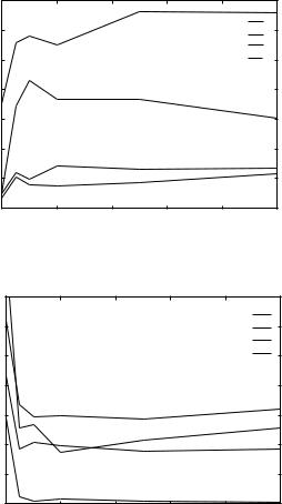
We address the convergence of the Z score in Fig. 6. How many shuffled sequences do we need before we get a reliable estimate? For example, after 100 shuffles the Z score of the global alignment of 1pbxA into 2lig (two different families) suggests that the result is significant. However, enlarging the sample to include 1000 random probes significantly reduces the Z score below the ‘‘cutoff’’ of 3. Hence, especially when the signal is not very strong, it is important to fully converge the value of the Z score. The large number of alignments that are performed for the shuffled sequences (between 50 and 1000) makes the process computationally demanding and underlines the need of an efficient algorithm for genomics scale threading experiments.
An essential decision needed is what is a ‘‘good’’ score and what is a ‘‘bad’’ score. Intuitively, negative energies are assumed ‘‘good.’’ Negative energies are lower than the state with no contacts—that is, contacts with water molecules as in the unfolded state. However, no such intuition is obvious for the Z score. To establish a cutoff for the Z score that eliminates false positives, we consider the probability PðZpÞ of observing a Z score larger than Zp by chance. Clearly our
110 |
jaroslaw meller and ron elber |
|
4.5 |
|
|
|
4 |
|
2lig |
|
|
1babB |
|
|
|
|
|
|
|
|
1pbxA |
|
3.5 |
|
1pbxB |
Z score |
3 |
|
|
2.5 |
|
|
|
|
2 |
|
|
|
1.5 |
|
|
|
1 |
600 |
1000 |
|
200 |
Number of alignments for randomly shuffled sequences
|
|
(a) |
|
|
4.5 |
|
|
|
4 |
|
2lig |
|
|
7acn |
|
|
|
|
1gky |
|
3.5 |
|
1pbxA |
Z score |
3 |
|
|
2.5 |
|
|
|
|
2 |
|
|
|
1.5 |
|
|
|
1 |
600 |
1000 |
|
200 |
Number of alignments for randomly shuffled sequences
(b)
Figure 6. The convergence of the Z scores as a function of the number of shuffled sequences. The results for global and local alignments are presented in the parts a and b, respectively. The sequence of the aspartate receptor protein 2lig (not included in the training set) is aligned to all the structures of the HL set, and the best matches are shown. Note that hemoglobin 1pbxA is found among the good matches (false positive) with a global Z score of about 3 when using only 100 shuffled sequences to estimate the distribution for random sequences. Converging the Z scores makes it possible to better separate the native alignment with respect to incorrect alternatives. The Z score for local alignment of 2lig into 1pbxA is small (about 1) and suggests that this match is indeed a false positive. The initial values in the figure correspond to scaled energies of the alignments.
protein recognition by sequence-to-structure fitness |
111 |
results will be statistically significant only if PðZpÞ is very small. The expectation value of the number of occurrences of false positives in N alignments with a Z score larger than Zp is N PðZpÞ.
To estimate PðZpÞ, we thread sequences of the S47 set through structures included in the Hinds–Levitt set. The probe sequences of known structures were selected to ensure no structural similarity between the HL set and the structures of the probe sequences (see Section III.A). Therefore any significant hit in this set may be regarded as a false positive.
Z scores of local alignments are employed to estimate PðZpÞ. In local alignments the number of ‘‘good’’ energies (significantly lower than zero) is large, underlining the need for an additional selection mechanism to eliminate false positives. It also makes it possible for us to estimate PðZpÞ for a population of alignments with ‘‘good’’ scores. For each probe sequence, Z scores are calculated for 200 structures with the best energies. Only alignments with matching segments of at least 60% of the total sequence length are considered. One hundred shuffled sequences are used to compute the averages required for a single Z-score evaluation. A histogram of the resulting 6813 pairwise alignments is presented in Fig. 7.
800 |
|
|
|
|
|
|
|
700 |
|
|
|
|
|
|
|
600 |
|
|
|
|
|
|
|
500 |
|
|
|
|
|
|
|
400 |
|
|
|
|
|
|
|
300 |
|
|
|
|
|
|
|
200 |
|
|
|
|
|
|
|
100 |
|
|
|
|
|
|
|
0 |
−3 −2 −1 |
0 |
1 |
2 |
3 |
4 |
5 |
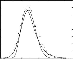
Figure 7. The probability distribution function of the Z scores computed for the population of false positives. A set of 47 sequences from the 547 set of proteins with known structures without homologs in the HL set is used to sample the distribution of Z scores for false positives. Each of the sequences is aligned to all the structures included in HL set. The Z scores are calculated for the 200 best matches (according to energy) using 100 shuffled sequences. The observed distribution of Z scores is represented by þ. The dashed line shows the attempted analytical fit to a Gaussian distribution, whereas the solid line the analytical fit to the expected extreme value (double exponential) distribution. Note the significant tail to the right, which is the probability of obtaining a relatively large Z score by chance. See text for more details.
112 |
jaroslaw meller and ron elber |
Let us denote by ^pðZÞ the probability density of findingÐ a Z-score value
between Z and Z þ dZ. Hence, PðZpÞ is given by PðZpÞ ¼ 1Zp ^pðZÞ dZ. We approximate the observed distribution (‘þ’) by an analytical fit to the extreme
value distribution (represented by a continuous line in Fig. 6), which is defined by [55]
^pðZÞ ¼ 1=s exp½ ðZ aÞ=s eðZ aÞ=s& |
ð16Þ |
In the realm of sequence comparison, the extreme value distribution has been used to model scores of random sequence alignments for local, ungapped alignments [56] as well as for local alignments with gaps [57].
The observed distribution is asymmetric and has a long tail toward high Z-score values (which is the tail that we are mostly interested in). Note, however, that there are significant differences between the numerical data and the analytical fit (and of course from the symmetric Gaussian distribution; dotted line in Fig. 7). Some deviations are expected because the distribution we extracted numerically differs from a random distribution. As discussed above, we use, for example, only alignments with negative energies. Hence, the energy filter was already employed.
Using analytical fit, we find that PðZpÞ ¼ 1 exp½ expð 1:313 ðZp þ 0:466ÞÞ& with the 98% confidence intervals 1:313 0:112 and 0:466 0:079. For example, we estimate that the probability of observing a random Z score that is larger than 4 is 0.003. We emphasize, however, that the analytical fit is an upper bound as is shown in Fig. 6. For example, the observed number of Z scores larger than 4.0 is equal to 3—as opposed to the expected number of finding a Z score larger than 4.0, which is equal to (according to the analytical fit) 6813 0:003 ¼ 20:4.
We observe similar discrepancy for global threading alignments of all the sequences from the HL set into all the structures in the HL set. For each probe sequence we select the 10 best matches (with lowest energies) that are subsequently subject to the statistical significance test, resulting in a sample of 2460 Z scores. Only five of the calculated Z scores, which are larger than 3.0, correspond to false positives. Using the analytical fit from Fig. 7 the expected number of observing by chance Z scores larger than 3.0 is equal to 24.6. Thus, it seems that the conservative estimate of the tail of the extreme value distribution indeed provides an upper bound for the probability of observing a false positive with a low energy and a high Z score.
B.Double Z-Score Filter
When searching large databases, the probability of observing false positives is growing, because the expected number of false positives is N PðZpÞ, where N is the number of structures in the database. Therefore, only relatively high Z
protein recognition by sequence-to-structure fitness |
113 |
scores may result in significant predictions. Unfortunately, there are many correct predictions with low Z scores that overlap with the population of false positives. A high cutoff will therefore miss many true positives. Restricting the Z score test to only best matches (according to energy) is still insufficient. Therefore we propose an additional filtering mechanism, based on a combination of Z scores for global and local alignments. The double Z-score filter eliminates false positives, missing much smaller number of correct predictions.
Global alignments (in contrast to local alignments) are influenced significantly by a difference in the lengths of the structure and the threaded sequence. The matching of lengths was considered too restricted in previous studies [58]. However, at our hands and using environment-dependent gap penalty, the Z
Local
10
9 8 7
6
5
4 3 2
1
0
−1 −2
−3−3 −2 −1 0 1 2 3 4 5 6 7 8 9 10 Global
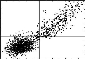
Figure 8. The joint probability distribution for the Z scores of global and local alignments. The distribution at the lower left corner (circles) is the result of the alignments of the 547 set sequences against all structures in HL set. The Z scores for the false positives are computed using 1000 shuffled sequences for both global and local alignments to ensure convergence. Only weak energy constraint are used; that is, 100 best global and 200 best local matches are subject to a Z score test, and then a given pair (global Z score, local Z score) is included if the energy of the global alignment is negative. The resulting 1081 pairs are included in the figure. The best pair in this population is slightly below the threshold (3.0,2.0). The population in the right upper corner represents (square boxes) 331 pairs of HL sequences aligned to HL structures with global Z scores larger than 2.5 and local Z scores larger than 1 [some of the Z scores fall beyond the (10,10) range). This set includes 236 native alignments and 95 non-native alignments. There are 10 matches that are false positives (filled squares), and they are all below the threshold (3, 2). Four of them are marginally so. The Z scores of this distribution were generated using 1000 shuffled sequences for global alignments, but only 50 for local alignments. Stiffer energy constraints were employed in which only the 10 best matches (according to energy) for global alignments and with 200 best matches for local alignments were considered. Of course, there is still a population of matches below (2.5,1.0) threshold (including 10 native alignments). However, the number of false positives below this threshold grows quickly, making predictions with Z scores in this range difficult.
114 |
jaroslaw meller and ron elber |
score of the global alignment was proven a useful independent filter. This filter is an addition to the use of energy (of local and global alignments) and of the Z score of local alignments.
In Fig. 8 we present the joint probability distribution for global and local Z scores for a population of false positives versus a population of correct predictions. The squares at the upper right corner represent correct predictions, resulting from 331 native alignments (of a sequence into its native structure) and homologous alignments (of a sequence into a homologous structure) of the HL set proteins. The circles at the left lower corner are false positives obtained from the alignments of the sequences of the S47 set against all structures in the HL. The procedure is the same as the one used previously to generate the probability density function for the Z scores of local alignments (see Fig. 7). However, the Z scores are computed using 1000 shuffled sequences for both global and local alignments, which is sufficient to converge the values of the Z scores. The converged results reduce somewhat the tails of the distribution. For example, the number of false positives with a global Z score larger than 2.5 and a local Z score larger than 1.0 is equal to 3, as compared to 7 with only 100 shuffled sequences.
Figure 8 shows that the thresholds of 3.0 for global Z scores and of 2.0 for local Z scores are sufficient to eliminate all the false predictions. These cutoffs result in a number of misses, for example, 23 native alignments are dismissed as insignificant (see also the next section). However, this is a price we have to pay for high confidence levels in our predictions. The total number of pairwise alignments for which we compute the global and the local Z scores, and subsequently test for the presence of false positives, is about 10,000. Hence, we estimate that the probability of observing a single false positive with a global and a local Z score larger than the 3.0 and 2.0 thresholds is smaller than 0.0001.
VII. TESTS OF THE MODEL
There are three tests that we perform in this section on the THOM2 potential. We use optimal alignments and the double Z-score test proposed in Section VI. First, we analyze the results of threading the sequences of the HL set into all the structures of the HL set. Self-recognition and family recognition are discussed. Next, threading of the CASP3 sequences into an extended TE set is used to test the performance of the new threading protocol on the set of folds that were not included in the training. Finally, further tests of family recognition are presented, including the comparison of THOM2 results with those of a pairwise model using the frozen environment approximation.
A.The HL Test
The HL set was partially learned (using gapless threading). The first test verifies that the additional flexibility of gaps and deletion maintain good prediction