

Friesner R.A. (ed.) - Advances in chemical physics, computational methods for protein folding (2002)(en)
.pdfsubject index |
525 |
Simulation errors, tertiary protein structure, ab initio folding potential predictions, 227–230
Single-descriptor models, protein folding statistical analysis, 16–19
linear correlations, 16
neural network predictions, 16–19 Single-domain proteins:
folding kinetics, 36–38
native vs. decoy protein conformations, 472–474
Single-step potentials, protein recognition, THreading Onion Model (THOM), 81–83
Site mapping, protein-protein interactions, binding affinity prediction, 413–414
Size-dependent potential energy function, tertiary protein structure, ab initio predictions, folding potential, 226–237
error identification, 226–230 improvements in, 230–233
PDB-derived secondary structure, 241–245 results, 233–237
Smith-Waterman algorithm, THOM2 model vs. pair energies, 120–126
Solvation energy models:
native vs. decoy protein conformations: Coulomb approximation, dielectric models,
478–480
research background, 460–462 oligopeptide structure prediction, 291–296
computational studies, 301–312 protein-protein interactions, binding site
structure prediction, 416–418, 437–438 Sparse restraints, structural refinement,
336–359
algorithmic steps, 345–347 computational study, 347–353
DYANA vs. torsion angle dynamics (TAD), 353–356
energy modeling, 339–341 global optimization, 341
torsion angle dynamics (TAD), 341–345, 356–359
Square well potential (SWP), capacity comparisons of new models, 93–100
Stationary points, protein folding mechanism: clustering algorithm, 396–397 eigenmode-following search, 392–393
fill algorithm, 395–396
Grid search, 394
research framework, 391–393 searching strategies, 365–366 SUMSL algorithm, 393 triples search, 395
unsolvated tetra-alanine, 370–371 uphill search, 394–395
Statistical analysis, protein folding kinetics: folding rates, 9–26
database, 11–16 multiple-descriptor models, 19–24 physical observations, 24–26 review, 9–11
single-descriptor models, 16–19 homologous proteins, 28–29 lattice models, 6–8
protein and lattice model studies, 29–30 research background, 2–3
techniques, 3–6 unfolding rates, 26–28
Structure prediction techniques: polypeptides:
computational models, 301–312 free energy computational studies,
322–336
free energy modeling, 312–314
global optimization framework, 296–300 harmonic approximation, 314–318
local minimum energy conformation, 318–322
potential energy models, 288–291 solvation energy models, 291–296 sequence-structure-function paradigm,
147–148
tertiary protein structure, knowledge-based prediction, 214–218
identification, 215
local templates, 217–218 multiple templates, 215–217
Substrate protein (SP), chaperonin-facilitated protein folding mechanism, 64–66
stretching-induced unfolding, 68–69 SUMSL algorithm, protein folding, stationary
points searching, 393
Surface formulation of generalized Born model (SGB), native vs. decoy conformations:
applications, 483–484
approximate effective dielectric models: distance-dependent dielectric
approximation, 480–481
526 |
subject index |
Surface formulation of generalized Born model (SGB), native vs. decoy
conformations: (Continued) screened Coulomb approximation,
478–480
CASP3 targets, 473–474 decoy data sets, 464–465 energy components, 474–478
force feld calculations, 462–464
Holm and Sander single decoys, 472–473 interior dielectric constant, 481–482 Park and Levitt decoys, 465–472 research background, 460–462
Template competition, tertiary protein structure, 216
Tendamistat (3AIT), tertiary protein structure, distance constraints, 206–207
TE potential:
capacity comparisons of new models, 93–100 distance power-law potentials, 92–93 energy parameter optimization, 87–88 minimal models, 91–92
native alignments in, 98–100 parameter-free optimization, 90–91 THOM2 model vs. pair energies, 125–126
Terminal loops, tertiary folding simulation, secondary structure definition and truncation, 245
Tertiary contacts, sequence-structure-function prediction:
restrained lattice folding, 158–159 threading-based prediction, 153–155
Tertiary protein structure:
ab initio predictions, folding potential: PDB-derived secondary structure
simulations, 238–246 methodology, 238–241 size-dependent potential, 241–245
terminal loop definition and truncation, 245
three-dimensional topologies, 245–246 predicted-derived secondary structure
simulations, 246–260 research background, 224–226
size-dependent potential energy function, 226–237
error identification, 226–230 improvements in, 230–233 results, 233–237
knowledge-based prediction: constraint methods, 201–210
ambiguous constraints, 205, 208–209 angle constraints, 202, 207–208 distance constraints, 202, 206–207 implementation, 204–205 predictions, derivation from, 203–204,
209–210
constraint refinement, 219 homology and structural templates,
214–218 identification, 215
local templates, 217–218 multiple templates, 215–217
protein modeling, 197–201 computational models, 197–198 geometrical representations, 198–199 scoring functions, 200–201
search algorithms, 199–200 research issues, 194–197
search space limitation, 210–214 fragment screening and enrichment,
212–213
local threading and fragment lists, 211–212
secondary structure modeling, 213–214 threading principle, 210–211
sequence-specific potentials, 218–219 Tetra-alanine:
coil-to-helix transition, 370–371 pathway determination, 374–378 rate disconnectivity graph, 378–380
protein folding, coil-to-helix transition, solvated model, 386–390
Thermodynamic hypothesis:
protein folding mechanisms, 268–269 sequence-structure-function prediction,
144–146
tertiary protein structure, computational modeling, 197–198
THreading Onion Model 1 (THOM1): capacity comparisons, 93–100 dissection of potential, 94–100 energy parameter optimization, linear
programming, 88–89 energy profiles, 83–85
gap energy training, 104–107 minimal models, 91–92 pairwise models, 81–83 parameter-free models, 90–91
subject index |
527 |
THreading Onion Model 2 (THOM2): capacity comparisons, 93–100, 98–100 energy profiles, 83–85
gap energy training, 104–107 minimal models, 91–92 pairwise models, 81–83 testing of, 114–126
HL test, 114–118
protein recognition excluded from training, 118–120
vs. pair energies, 120–126 Threading protocols:
comparison of potentials, 91–92
linear programming (LP) protocol, 101–102 protein recognition, 78–79 sequence-structure-function prediction,
134–138, 147
biochemical function prediction, 175–178 first-pass threading, 148–149
Fischer database applications, 149–151 genome-scale iterative threading, 152–153 iterative threading, 151–152 orientation-dependent pair potential,
PROSPECTOR extension, 153 tertiary contacts, 153–155
tertiary protein structure, search space limitation, knowledge-based prediction, 210–211
local threading and fragment lists, 211–212 THOM2 model, HL test, 114–118
Three-descriptor models, protein folding kinetic statistical analysis, 22–24
Time-dependent probabilities, protein folding, potential energy surfaces, 399–400
Time-evolution of quantities, protein folding, coil-to-helix transition, 380–382
Topological frustration, protein folding mechanisms, 52–53
Torsional energy expressioin, oligopeptide structure prediction, potential energy models, 289–291
Torsion angle dynamics (TAD), sparse restraints, structural refinement, 338–359
algorithmic steps, 345–347 global optimization, 356–359 molecular dynamics, 341–345 vs. DYANA protocol, 353–356
Total energy profile, protein recognition, 83–85
Transition rate cutoff, protein folding:
coil-to-helix transition pathways, 374–378 potential energy surface calculation, 399 Transition states, protein foldinig, minima and first-order algorithms, 393–397
Translation vector, protein-protein interactions, binding site structure prediction,
432–435
Triose phosphate isomerase (TIM), sequence- structure-function prediction, 172
Triples algorithm, protein folding: potential energy surfaces, 366–367 stationary points searching, 395
Twice continuously differentiable NLPs, deterministic global optimization, 269–279
aBB algorithm, 276–279 convex lower bounding, 275
feasible region convexification, 274–275 nonconvex terms, underestimation, 272–274 special structure, underestimation, 270–272 variable bound updates, 275–276
Two-descriptor models, protein folding kinetic statistical analysis, 20–22
Two-state protein folding: kinetics, 37–38 mechanisms, 49–51
Underestimating problems, deterministic global optimization, twice continuously differentiable NLPs, aBB algorithm, 277–279
Unfolding rates:
chaperonin-facilitated protein folding mechanism, 66–67
stretching techniques, 68–69
protein folding statistical analysis, 26–28 Unified folding method, sequence-structure- function prediction, 146–148
Univariate concave functions, deterministic global optimization, twice continuously differentiable NLPs, 270–272
Uphill search algorithm, protein folding, 394–395
Upper bound check (UBC), oligopeptide structure prediction:
global optimization, 299–300
local minimum energy conformations, 320–321
Urey-Bradley distance, potential energy surface, 404–405
528 |
subject index |
Van der Waals interactions:
native vs. decoy protein conformations, 476–478
oligopeptide structure prediction, potential energy models, 290–291
Variable bound updates, deterministic global optimization, twice continuously differentiable NLPs, 275–276
aBB algorithm, 276–279 Vibrational frequencies, protein folding
mechanism, potential energy surface, 397–398
Zero-parameter models, optimization, 90–91
Zimmerman codes, oligopeptide structure prediction, computational studies, 325–336
Z-score filter:
energy gap alignments, 108–112
native vs. decoy protein conformations, Park and Levitt decoys, 468–472
THOM2 model: HL test, 114–118
vs. pair energies, 120–126
Computational Methods for Protein Folding: Advances in Chemical Physics, Volume 120.
Edited by Richard A. Friesner. Series Editors: I. Prigogine and Stuart A. Rice. Copyright # 2002 John Wiley & Sons, Inc.
ISBNs: 0-471-20955-4 (Hardback); 0-471-22442-1 (Electronic)
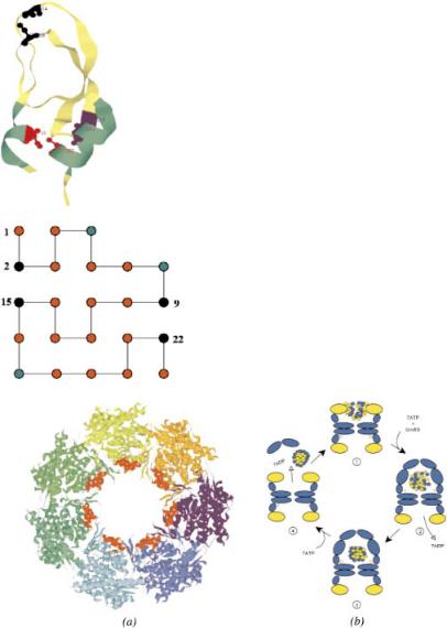
Figure 7. (See Chapter 2.) The native-state conformation of the bovine pancreatic trypsin inhibitor (BPTI). The figure was produced with the program RasMol 2.7.1 [126] from the PDB entry 1bpi. There are three disulfide bonds in this protein: Cys5–Cys55 shown in red, Cys14–Cys38 shown in black, and Cys30–Cys51 shown in blue. The corresponding Cys residues are in the ball-and-stick representation and are labeled. The two helices (residues 2–7 and 47–56) are shown in green.
Figure 8. (See Chapter 2.) (a) The ground-state conformation of the two-dimensional model sequence with M ¼ 23 beads and four covalent (S) sites. The red, green, and black circles represent, respectively, the hydrophobic (H), polar (P), and S sites.
Figure 9. (See Chapter 2.) (a) Rasmol [126] view of one of the two rings of GroEL, from the PDB file 1oel. The seven chains are indicated by different colors. The amino acid residues forming the binding site of the apical domain of each chain (199–204, helix H: 229–244 and helix I: 256– 268) are shown in red. The most exposed hydrophobic amino acids that are facing the cavity and are implicated in the binding of the substrate as indicated by mutagenesis experiments [112, 127] are: Tyr199, Tyr203, Phe204, Leu234, Leu237, Leu259, Val263, and Val264. (b) A schematic sketch of the hemicycle in the GroEL–GroES-mediated folding of proteins. In step 1 the substrate protein is captured into the GroEL cavity. The ATPs and GroES are added in step 2, which results in doubling the volume, in which the substrate protein is confined. The hydrolysis of ATP in the cis-ring occurs in a quantified fashion (step 3). After binding ATP to the trans-ring, GroES and the substrate protein are released that completes the cycle (step 4).
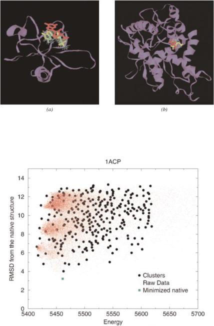
Figure 4. (See Chapter 4.) For the predicted protein structure of 2sarA (2cmd_) generated by GeneComp using a template provided by the Fischer Database [34], the red-colored ligand represents the superposition of the ligand bound to the native receptor. The highest-scored match is colored in yellow.
Figure 7. (See Chapter 6.) Comparison of raw data and clustered results (red dots: raw simulation data, black circles: cluster representatives, green square: locally minimized native structure).
Computational Methods for Protein Folding: Advances in Chemical Physics, Volume 120.
Edited by Richard A. Friesner. Series Editors: I. Prigogine and Stuart A. Rice. Copyright # 2002 John Wiley & Sons, Inc.
ISBNs: 0-471-20955-4 (Hardback); 0-471-22442-1 (Electronic)
STATISTICAL ANALYSIS OF PROTEIN
FOLDING KINETICS
AARON R. DINNER
New Chemistry Laboratory, University of Oxford, Oxford, U.K.
SUNG-SAU SO
Hoffmann-La Roche Inc., Discovery Chemistry, Nutley, NJ, U.S.A.
MARTIN KARPLUS
New Chemistry Laboratory, University of Oxford, Oxford, U.K.; Department of Chemistry and Chemical Biology, Harvard University, Cambridge, MA, U.S.A.; and Laboratoire de Chimie Biophysique, Institut le Bel,
Universite´ Louis Pasteur, Strasbourg, France
CONTENTS
I.Introduction
II. Statistical Methods III. Lattice Models
IV. Folding Rates of Proteins
A.Review
B.Database
C.Single-Descriptor Models
1.Linear Correlations
2.Neural Network Predictions
D.Multiple-Descriptor Models
1.Two Descriptors
2.Three Descriptors
E.Physical Bases of the Observed Correlations
1
2 |
aaron r. dinner et al. |
V. Unfolding Rates of Proteins
VI. Homologous Proteins
VII. Relating Protein and Lattice Model Studies
VIII. Conclusions
Acknowledgments
References
I.INTRODUCTION
Experimental and theoretical studies have led to the emergence of a unified general mechanism for protein folding that serves as a framework for the design and interpretation of research in this area [1]. This is not to suggest that the details of the folding process are the same for all proteins. Indeed, one of the most striking computational results is that a single model can yield qualitatively different behavior depending on the choice of parameters [1–3]. Consequently, it remains to determine the behavior of individual sequences under given environmental conditions and to identify the specific factors that lead to the manifestation of one folding scenario rather than another. Although doing so requires investigation of the kinetics of particular proteins at the level of individual residues, for which protein engineering [4] and nuclear magnetic resonance (NMR) [5] experiments are very useful, complementary information about the roles played by the sequence and the structure can also be obtained by a statistical analysis of the folding rates of a series of proteins.
Statistical methods have been applied for many years in attempts to predict the structures of proteins (for a review of progress in this area, see the chapter by Meller and Elber, this volume), but their use in the analysis of folding kinetics is relatively recent. The first such investigations focused on ‘‘toy’’ protein models in which the polypeptide chain is represented by a string of beads restricted to sites on a lattice. It was found that the ability of a sequence to fold correlates strongly with measures of the stability of its native (ground) state (such as the Z-score or the gap between the ground and first excited compact states) [6–9], but the native structure also plays an important role for longer chains [10,11]. While lattice models are limited in their ability to capture the structural features of proteins, they have the important advantage that the results of statistical analyses can be compared with calculated folding trajectories to determine the physical bases of observed correlations. Consequently, studies based on such models are particularly useful for the quantitation of observed effects, the generalization from individual sequences, the identification of subtle relationships, and ultimately the design of additional sequences that fold at a given rate.
Analogous statistical analyses of experimentally measured folding kinetics of proteins were hindered by the fact that complex multiphasic behavior was exhibited by most of the proteins for which data were available (e.g., barnase and lysozyme). In recent years, an increasing number of proteins that lack
statistical analysis of protein folding kinetics |
3 |
significantly populated folding intermediates and thus exhibit two-state folding kinetics have been identified, and a range of data have been tabulated for them [12–14]. The initial linear analyses of such proteins indicated that their folding rates are determined primarily by their native structures [12,14]. More recently, a nonlinear, multiple-descriptor approach revealed that there is a significant dependence on the stability as well [15]. These and related studies are discussed in Section IV.A, after an overview of the statistical methods employed in this area (Section II) and a review of the results from lattice models (Section III).
An in-depth analysis of a database of 33 proteins that fold with twoor weakly three-state kinetics is presented in Sections IV.B through V. We explore one-, two-, and three-descriptor nonlinear models. A structurally based crossvalidation scheme is introduced. Its use in conjunction with tests of statistical significance is important, particularly for multiple-descriptor models, due to the limited size of the database. Consistent with the initial linear studies [12,14], it is found that the contact order and several other measures of the native structure are most strongly related to the folding rate. However, the analysis makes clear that the folding rate depends significantly on the size and stability as well. Due to the importance ascribed to the stability by analytic [16–18] and simulation [2,3,6–11] studies, as well as its recent use in one-dimensional models for fitting and interpreting experimental data [19,20], we examine its connection to the folding rate in more detail. The unfolding rate, which correlates more strongly with stability, is considered briefly. The relation of the statistical results to experiments and the model studies is discussed in Sections VI and VII.
II.STATISTICAL METHODS
Before reviewing the results for specific systems, we introduce the statistical methods that have been used to analyze folding kinetics. Perhaps the simplest such method is to group sequences; here, one categorizes each sequence in a database according to one or more of its native properties (‘‘descriptors’’) and its folding behavior. Visualization can be used to identify patterns, and averages and higher moments of the distributions of descriptors can be used to quantitate differences between groups. For properties on which the folding kinetics depend strongly, such as the energy gap in lattice models, this type of analysis has proven effective [6].
However, simple grouping is often insufficient to identify weaker but still significant trends and makes it difficult to determine the relative importance of relationships. Consequently, more quantitative methods are necessary. One statistic that is employed widely is the Pearson linear correlation coefficient (rx;yÞ:
rx;y |
|
sxy2 |
Piðxi xÞðyi |
|
yÞ |
|
1 |
|||||
|
|
|
|
q i i i i |
|
|||||||
|
¼ sxsy ¼ |
P ð |
x |
x |
2 |
P |
y |
|
y 2 |
ð Þ |
||
|
|
|
|
|
Þ |
|
ð |
Þ |
|
|||

4 |
aaron r. dinner et al. |
Typically, the xi are a set of values of a particular descriptor, such as the sequence length, and the yi are a set of values for a measure of the folding kinetics, such as the logarithm of the folding rate constant (log kf ) [9,10,12]. The magnitude of rx;y determines its significance, and its sign indicates whether xi and yi vary in the same or opposite manner: rx;y ¼ 1 corresponds to a perfect correlation, rx;y ¼ 1 to a perfect anticorrelation, and rx;y ¼ 0 to no correlation. In spite of its popularity, this statistic has several shortcomings when used by itself. It is limited to the identification of linear relationships between pairs of properties; it is not straightforward to test or cross-validate those relationships, which is important, as discussed below; and it cannot be used directly to predict the behavior of additional sequences.
These limitations can be overcome by constructing models to predict folding behavior and then quantifying their accuracy. For the latter step, the Pearson linear correlation coefficient can be used with xi as the observed values and yi as the predicted ones (for which we introduce the shorthand notations rtrn, rjck, and rcv, described below). Alternatively, one can calculate the root-mean-square error or the closely related fraction of unexplained variance:
q2 |
¼ |
1 |
Piðyi xiÞ2 |
2 |
Þ |
|
|
Piðxi xÞ2 |
ð |
Again, xi (yi) are the observed (predicted) values. Typically, r and q2 behave consistently. The latter is useful for quantitating the improvement obtained upon extending a model with N descriptors to one with N þ 1 with Wold’s statistic: E ¼ ð1 q2Nþ1Þ=ð1 q2N Þ [21,22]. A value of less than 1.0 for the latter shows that q2 increases upon adding a descriptor. The statistical significance of a particular value of E depends on the specific data, but E ¼ 0:4 has been suggested to correspond typically to the 95% confidence interval [23].
For constructing the models themselves, linear regression (on one or more descriptors) is attractive in that the best fit for a set of data can be determined analytically, but, as its name implies, it is limited to detecting linear relationships. While fits with higher-order polynomials are possible, a general and flexible alternative is to use neural networks (NNs). The latter are computational tools for model-free mapping that take their name from the fact that they are based on simple models of learning in biological systems [24,25]. Neural networks have been used extensively to derive quantitative structure–property relationships in medicinal chemistry (for a review, see Ref. 26) and were first used to analyze folding kinetics in Ref. 11. A schematic diagram of a neural network is shown in Fig. 1. In this example, there are three inputs (indicated by the rectangles on the left); in the present study these would each contain the value of a descriptor, such as the free energy of unfolding or the fraction of