Friesner R.A. (ed.) - Advances in chemical physics, computational methods for protein folding (2002)(en)

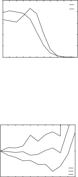
during the process of learning. As a result, the LP has the potential for accumulating more information, attempting to put the energies of the misthreaded sequence as far as possible from the correct thread. In Fig. 4 we show the results of the LP training for valine, alanine, and leucine that are in general agreement with the statistical data above. Nevertheless, some interesting and

0 1 2 3 4 5 6 7 8 9 10 11 Number of contacts

(b)

Figure 3. Statistical analysis of contacts for the THOM1 model. (a) Distribution of the number of contacts for hydrophobic residues. (b) Distribution of the number of contacts for (c) Data for alanine and glycine.

significant differences remain. For example, very rare valine residues with 10 neighbors obtain positive energies.

A plausible interpretation of this result is that these rare sites are used to enhance recognition in some cases, due to specific ‘‘homologous features.’’ In Table Va we examined the type of contacts (in terms of the number of neighbors) for native and decoy structures.

Number of contacts

Figure 4. Potentials for THOM1 energy as extracted from LP training. Three residues are shown: alanine, lysine, and valine. Note that the minimum of the potential for valine is at seven neighbors. Note also that lysine has a minimum at zero neighbors.

aFrequencies of different types of sites (relevant for the training of THOM1) found in the native structures of HL set as opposed to decoy structures generated using the HL set are presented in part a. In THOM1 the type of site is defined by number of its neighbors (n). Frequencies are defined by the percentage from the total number of 53,012 native sites in HL set and 556.14 millions of decoy sites generated using HL set, respectively. Frequencies of different types of contacts (appropriate for the training of THOM2) found in the native structures of TE set as opposed to decoy structures generated using TE are given in Table Vb. Different classes of contacts are specified in Table II. Frequencies are defined by the percentage from the total number of 439,364 native contacts in TE set and 10,089.19 millions of decoy contacts generated using TE set, respectively. The comparable site and contact distributions separated for hydrophobic and polar residues (as defined in Table I) are given in parentheses.

It is evident that native structures tend to have more contacts but that the difference is not profound. The deviations are the result of threading short sequences through longer structures (we have more threading of this kind). Such threading suggests a small number of contacts for the set of decoy structures. A sharper difference between native and decoy structures is observed when the contacts are separated to hydrophobic and polar (Table Vb). The difference in hydrophobic and polar contacts is very small at the decoy structures and much more significant for the native shapes.

Another reflection of the same phenomenon is the statistics of pair contacts. For the native structures we find that 42.6% of the contacts are of HH type, 38.2% are HP, and 19.3% are PP. This statistics is of the HL set that has a total of 93,823 contacts. For the decoy structures the statistics of pair contacts is vastly different. Only 23.5% of the contacts are HH, HP contacts are 50% of the total, and 26.5% are PP. The number of contacts that were used is 833.79 million. More details can be found in Tables Va and Vb.

THOM2 has significantly higher capacity, however the double layer of neighbors makes the results more difficult to understand. In Fig. 2 we showed the energy contributions of a few typical structural sites as defined by the THOM2 model. For example, the ‘‘lowest’’ picture in Fig. 2 is a site with six neighbors in the first contact shell and a wide range of neighbors in the second shell. The second shell includes a site with just two neighbors as well as a site with nine neighbors. The overall large number of neighbors suggests that this site is hydrophobic, and the corresponding energies of lysine and valine indeed support this expectation.

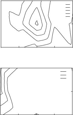
In Fig. 5 we present a contour plot of the total contributions to the energies of the native alignments in the TE set, as a function of the number of contacts in the first shell, n, and the number of secondary contacts to a primary contact, n0, respectively. The results for two types of residues, lysine and valine, are presented. The contribution of a type of site to the native alignment is twofold: its energy eaðn; n0Þ and the frequency of that site f . It is possible to find a very attractive (or repulsive) site that makes only negligible contribution to the native energies because it is extremely rare (i.e., f is small). For specific examples see Table VI. By plotting f eaðn; n0Þ we emphasize the important contributions. Hydrophobic residues with a large number of contacts stabilize the native alignment, as opposed to polar residues that stabilize the native state only with a small number of neighbors.

It has been suggested that pairwise interactions are insufficient to fold proteins and higher-order terms are necessary [30]. It is of interest to check if the environment models that we use catch cooperative, many-body effects. As an example we consider the cases of valine–valine and lysine–lysine interactions. We use Eq. (8) to define the energy of a contact. In the usual pairwise

First shell

(a)

First shell

(b)

Figure 5. Contour plots of the total energy contributions to the native alignments in the TE set for valine and lysine residues as a function of the number of neighbors in the first and second shells. Part a shows that contacts involving valine residues with five to six neighbors with other residues of medium number of neighbors stabilize most the native alignments. On the other hand, as can be seen from part b, only contacts involving lysine residues with a small number of neighbors stabilize native alignments.

interaction the energy of a valine–valine contact is a constant and independent of other contacts that the valine may have.

In Table VI we list the effective energies of contacts between valine residues as a function of the number of neighbors in the primary and secondary sites. The energies differ widely from 1.46 to þ3.01. The positive contributions refer,

aFor a pair of two amino acids a and b in contact, we have 25 different possible types of contacts (and consequently 25 different effective energy contributions) because a and b may occupy sites that belong to one of the five different types characterized by the increasing number of contacts in the first contact shell (see Table II). Moreover, the 5 5 interaction matrix will, in general, be asymmetric. The effective energies of contact between two VAL residues with a different number of neighbors are given in part a, whereas the energies of contacts between two LYS residues are given in part b.

however, to very rare types of contacts, and the energies of the probable contacts are negative as expected. Hence, the THOM2 model is compensating for missing information on neighbor identities by taking into account significant cooperativity effects.

To summarize the study of the potentials we provide, in Table VII, the optimal parameters for LJ(6,2), THOM1, and THOM2 potentials.

V.THE ENERGIES OF GAPS AND DELETIONS

In the present section we discuss the derivation of the energy for gaps (insert-

ions in the sequence) and deletions. A gap residue is denoted by a , and a

¼ deletion is denoted by a v. For example, the extended sequence S

a1 va3 . . . an has a gap at the second structural position (x2) and a deletion at the second amino (a2).

A.Protocol for Optimization of Gap Energies

The gap (an unoccupied structural site) is considered to be an (almost) normal amino acid. We assigned to it a score (or energy) according to its environment, like any other amino acid. Here we describe how the energy function of the gap was determined. The parameters were optimized for THOM1 and THOM2, because these are the models accessible to efficient alignment with gaps.

Gap training is similar to the training of other amino acid residues. Only the database of ‘‘native’’ and decoy structures is different. To optimize the gap parameters we need ‘‘pseudo-native’’ structures that include gaps. We construct such ‘‘pseudo-native’’ conformations by removing the true native shape Xn of the sequence Sn from the coordinate training set and by putting instead a homologous structure, Xh. The best alignment of the native sequence into the

homologous structure is Sn into Xh, and it includes gaps. We require that the

TABLE VII

Parameters of Some of the Threading Potentials Trained Using the LP Protocola

(a)

alignment Sn into the homologous protein will yield the lowest energy compared to all other alignments of the set. Hence, our constraints are

X

ð Þ ð Þ ¼ ð ð Þ ð ÞÞ 8 ¼6

E Sn; Xj; p E Sn; Xh; p pg ng Xj ng Xh > 0 j h; n

g

ð13Þ

Equation (13) is different from Eq. (12) in two ways. First, we consider the

‘‘extended’’ set of ‘‘amino acids’’—S instead of S. Second, the native-like structure is Xh—a coordinate set of a homologous protein and not Xn.

The number of inequalities that we may generate (alignments with gaps inserted into a structure and deletions of amino acids) is exponentially large in the length of the sequence, making the exact training more difficult. Some compromises on the size of samples for inequalities with gaps have to be made. To limit the scope of the computations, we optimize here the scores of the gaps only. Thus, we do not allow the amino acid energies (computed previously by gapless threading; see Section III) to change while optimizing parameters for

gaps. Moreover, the sequence S (obtained by prior alignment of the native sequence against a homologous structure) is held fixed, and gapless threading against all other structures in the set is used to generate a corresponding set of

inequalities [Eq. (13)]. By performing gapless threading of Sn into different

structures, we consider only a small subset of all possible alignments of Sn, because we fixed the number and the position of the gaps that we added to the native sequence Sn.

Pairs of homologous proteins from the following families were considered in the training of the gaps: globins, trypsins, cytochromes and lysozymes (see Table VIII). The families were selected to represent vastly different folds with a

TABLE VIII

Pairs of Homologous Structures Used for the Training of Gap Penaltiesa

aFor each pair the native and the homologous structures are specified by their PDB codes, names, and lengths in the first and second column, respectively. In the third column the similarity between the native and the homologous proteins is defined in terms of sequence identity (%), RMS distance (angstroms), and length (number of residues) of the FSSP structure-to-structure alignment, obtained by submitting the corresponding pairs to the DALI server [44].

significant number of homologous proteins in the database. The globins are helical, trypsins are mostly b-sheets, and lysozymes are a/b proteins. Note also that the number of gaps differs appreciably from a protein to a protein. For example, Sn includes only one gap for the alignment of 1ccr (sequence) versus 1yea (structure), and 22 gaps for 1ntp versus 2gch.

The energy functional form that we used for the gaps is the same as for other amino acids. The ‘‘pseudo-native’’ structures with extended sequences are added to the HL set (while removing the original native structures). Gapless threading into other structures of the HL set results in about 200,000 constraints for the gap energies. Because we did not consider all the permutations of the gaps within a given sequence and our sampling of protein families is limited, our training for the gaps is incomplete. Nevertheless, even with this limited set we obtain satisfactory results. A representative set of homologous pairs that we used allows us to arrive at scores that can detect very similar proteins (e.g., the cytochromes 1ccr and 1yea) and also related proteins that are quite different (e.g., the globins 1lh2 and 1mba); see Table VIII.

The process of generating pseudo-native is as follows: For each pair of native

and homologous proteins the alignment of the native sequence Sn into the homologous structure Xh is constructed. This alignment uses an initial guess for the gap energy, which is based on the THOM1 potential and was based on the following observations.

*The gap penalty should increase with the number of neighbors. For example, we require that e ðn þ 1Þ > e ðnÞ for the THOM1 gap energy.

*The energy of a gap with contacts must be larger than the energy of an amino acid with the same number of contacts. The gap energy must be

higher; otherwise, gaps will be preferred to real amino acids. For example, the THOM1 energy of the proline residue with one neighbor is 0.29.

*The energy of amino acids without contacts is set to zero. The gap energy is therefore greater than zero.

In Table IX we provide the initial guess for the gaps (used to determine pseudo-native states) and the final optimal gap values for THOM1 and THOM2. The value of 10 is the maximal penalty allowed by the optimization protocol that we used. However, this value is not a significant restriction. A solution vector p can be used to generate another scaled solution lp, where l is a positive constant.

Nevertheless, note that the maximal value is reached rather quickly. This may indicate that our sampling of inequalities is still insufficient from the perspective of native alignment. The values of gaps that are found only in decoy states are increasing without limit in the LP protocol. For example, it is so rare