Добавил:

fench Опубликованный материал нарушает ваши авторские права? Сообщите нам.

Вуз:

Сумский государственный университет

Предмет:

Английский язык

Файл:

Dictionary of Geophysics, Astrophysic, and Astronomy.pdf

Скачиваний:

122

Добавлен:

10.08.2013

Размер:

5.66 Mб

Скачать

☆

►Содержание►

<<< < Предыдущая 21 22 23 24 25 26 27 28 29 30 31 3233 / 13033 34 35 36 37 38 39 40 41 42 43 44 45 > Следующая >>>

diffusion-convection equation

sionally, toward the second or higher diffraction orders. In this case, a grating is said to be blazed.

diffuse absorption coefﬁcient For downwelling (upwelling) irradiance: the ratio of the absorption coefﬁcient to the mean cosine of the downward (upward) radiance. See absorption coefﬁcient.

diffuse attenuation coefﬁcient For downwelling (upwelling) irradiance: the ratio of the sum of the absorption coefﬁcient and the scattering coefﬁcient to the mean cosine of the downward (upward) radiance.

diffuse aurora A weak diffuse glow of the upper atmosphere in the auroral zone, caused by collisions with the upper atmosphere of electrons with energies around 1 keV. It is believed that these electrons leak out from the plasma sheet of the magnetosphere, where they are trapped magnetically. The diffuse aurora is not conspicuous to the eye, but imagers aboard satellites in space see it as a “ring of ﬁre” around the magnetic pole. Discovered by ISIS-1 in 1972, its size, intensity, and variations — in particular, its intensiﬁcations and motions in substorms — are important clues to the state of the magnetosphere.

diffuse galactic light The diffuse glow observed across the Milky Way. A large part of the brightness of the Milky Way, which is the disk of our galaxy seen from the inside, can be resolved into stellar sources. The diffuse galactic light is a truly diffuse glow which accounts for the remaining 25% of the luminosity and, by deﬁnition, is unresolved even if observed with large telescopes. The diffuse galactic light is due to light emitted within our galaxy and scattered by dust grains, and it is not to be confused with light coming from extended sources like reﬂection or emission nebulae. The brightness close to the galactic equator due to diffuse galactic light is equivalent to 50 stars of 10th magnitude per square degree; for comparison, the total star background is 170 10th magnitude stars per square degree, and the zodiacal light 80.

diffuse interstellar bands (DIBs) A series of interstellar absorption features recorded on

photographic plates in the early 1900s. They were labeled “diffuse” because they arise from electronic transitions in molecules, so they are broad in comparison to atomic lines. There are now well over 100 such bands known in the UV, visible, and near IR regions of the spectrum arising in interstellar clouds. DIBs must be molecular, given the complexity of the absorption lines. DIBs are easily seen when observing spectra of hot, fast rotating stars whose spectrum has a strong continuum. Even with very high resolution spectroscopy, the diffuse interstellar bands continue to show blended structures. DIBs show considerable scatter in strength vs. the amount of stellar reddening suggesting inhomogeneous variation of chemistry and dust-to-gas ratio. This may arise because the molecule(s) in the volume may be able to add hydrogen to the molecular structure in certain circumstances, as is known for some carbon compounds. Identifying the carriers of these absorptions has become perhaps the classic astrophysical spectroscopic problem of the 20th century, and numerous molecules have been put forth as the source of these features. Recently most attention has focused on carbon rich molecules such as fullerenes and polycyclic aromatic hydrocarbons.

diffuse scattering coefﬁcient for downwelling (upwelling) irradiance The ratio of the scattering coefﬁcient to the mean cosine of the downward (upward) radiance.

diffusion The gradual mixing of a quantity (commonly a pollutant) into a ﬂuid by random molecular motions and turbulence.

diffusion-convection equation Transport equation for energetic charged particles in interplanetary space considering the effects of spatial diffusion and convection of particles with the solar wind. The transport equation can be derived from the equation of continuity by supplementing the streaming with the convective streaming vf , yielding

∂f + · (v sowif ) − · (D f ) = 0 ∂t

with f being the phase space density, D the (spatial) diffusion coefﬁcient, and v sowi the solar

diffusion creep

wind speed. The terms then give the convection with the solar wind and spatial scattering. The diffusion-convection equation can be used to model the transport of galactic cosmic rays or the transport of solar energetic particles beyond the orbit of Earth.

If v and D are independent of the spatial coordinate, the solution of the diffusionconvection equation for a δ-injection in the radial-symmetric case, such as the explosive release of energetic particles in a solar ﬂare, reads

	=	(4πDt)3	−	4Dt
f (r, t)		N o	exp	(r − vt)2	.
f (r, t)			exp		.

This latter equation is a handy tool to estimate the particle mean free path from intensitytime proﬁles of solar energetic particle events observed in interplanetary space, although for careful studies of propagation conditions numerical solutions of the complete transport equation should be used.

diffusion creep When macroscopic strain is caused by diffusion transport of matter between surfaces of crystals differently oriented with respect to differential stress, it is called diffusion creep. Nabarro–Herring creep, where vacancies diffuse through the grain between areas of its boundary, and Coble creep, where diffusion takes place along the grain boundary, are two examples. Diffusion creep results dominantly from the motions (diffusion) of species and defects (vacancies and interstitial). It is characterized by (1) a linear dependence of strain rate on stress (n = 1, n is stress sensitivity of creep rate at steady-state stage); (2) high grain-size sensitivity; (3) the rate-controlling species is the lowest diffusion species along the fastest diffusion path; (4) no lattice preferred orientation formed;

(5) little transient creep; (6) deformation is stable and homogeneous.

diffusion, in momentum space Momentum transfer between particles can be due to collisions as well as due to wave-particle interaction. If these collisions/interactions lead to energy changes distributed stochastically, and the energy changes in individual collisions are small compared to the particle’s energy, the process can be described as diffusion in momentum

space. Instead of the particle ﬂow considered in spatial diffusion, a streaming S p in momentum

results

∂f S p = −D pp ∂p

with p being the momentum, f the phase space density, and D pp the diffusion coefﬁcient in momentum.

Also if non-diffusive changes in momentum, e.g., due to ionization, can happen, the streaming in momentum can be written as

S p = −D pp	∂f	+	dp
				f
	∂p		dt

with the second term corresponding to the convective term in spatial diffusion. See diffusion- convection equation.

diffusion, in pitch angle space Waveparticle interactions lead to changes in the particle’s pitch angle. When these changes are small and distributed stochastically, diffusion in pitchangle space results. The scattering term can be derived strictly analogous to the one in spatial diffusion by just replacing the spatial derivative by the derivative in pitch-angle µ:

∂∂f

κ(µ)

∂µ ∂µ

with f being the phase space density and κ(µ) being the pitch-angle diffusion coefﬁcient. Note that κ depends on µ, that is scattering is different for different pitch-angles, depending on the waves available for wave-particle interaction. See resonance scattering, slab model.

diffusively stable A water column is called diffusively stable if both vertical gradients of salinity (β∂S/∂z) and of temperature (α∂?/∂z) enhance the stability N2 of the water column. The practical implication is that molecular diffusions of salt and temperature cannot produce local instabilities, as they can in double diffusion.

diffusive regime The diffusive regime is one of two possibilities, which allow double diffusion to occur. Under diffusive regimes, salinity stabilizes and temperature destabilizes the water column in such a way that the resulting vertical density proﬁle is stable, i.e.,

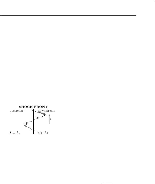
diffusive shock acceleration

Rρ =2	(β∂S/∂z)/(α∂?/∂z) > 1 (and stabil-
ity N	> 0).
diffusive shock acceleration		Acceleration

due to repeated reﬂection of particles in the plasmas converging at the shock front, also called Fermi-acceleration. Diffusive shock acceleration is the dominant acceleration mechanism at quasi-parallel shocks because here the electric induction ﬁeld in the shock front is small, and therefore shock drift acceleration is inefﬁcient. In diffusive shock acceleration, the scattering on both sides of the shock front is the crucial process. This scattering occurs at scatter centers frozen-in into the plasma, thus particle scattering back and forth across the shock can be understood as repeated reﬂection between converging scattering centers (ﬁrst order Fermi acceleration).

Particle trajectory in diffusive shock acceleration.

With f being the phase space density, U the plasma bulk speed, D the diffusion tensor, p the particle momentum, and T a loss time, the transport equation for diffusive shock acceleration can be written as

∂f

f )

∂f

∂t

−

+ T

3 ∂p

+p2

∂p p2

dt f

= Q(r, p, t)

∂

with Q(r, p, t) describing an injection into the acceleration process. The terms from left to right give the convection of particles with the plasma ﬂow, spatial diffusion, diffusion in momentum space (acceleration), losses due to particle escape from the acceleration site, and convection in momentum space due to processes that affect all particles, such as ionization or Coulomb losses.

In a ﬁrst-order approximation, the last two terms on the right-hand side (losses from the acceleration site and convection in momentum space) can be neglected. In addition, if we limit ourselves to steady state, some predictions can be made from this equation:

1. Characteristic acceleration time. With the indices u and d denoting the properties of the upstream and downstream medium, the time required to accelerate particles from momentum po to p can be written as

t = uu	3		p	p	·	u u	+ u d .
		ud
				dp		D u		Dd
	−		po

Here D denotes the diffusion coefﬁcient. Alternatively, a characteristic acceleration time τ a can be given as

τ a =	3r			D u
τ a =	r −	1		u2u

with r = u u/ud being the ratio of the ﬂow speeds in the shock rest frame. For a parallel shock, r equals the compression ratio. τ a then gives the time the shock needs to increase the particle momentum by a factor of e. Note that here the properties of the downstream medium have been neglected: It is tacitly assumed that the passage of the shock has created so much turbulence in the downstream medium that scattering is very strong and therefore the term D d/ud is small compared to the term D u/u u.

2. Energy spectrum. In steady state, diffusive shock acceleration leads to a power law spectrum in energy J (E) = Jo · E−γ . Here the spectral index γ depends on the ratio r = u u/ud of the ﬂow speeds only:

γ= 1 r + 2 2 r − 1

in the non-relativistic case, or γ rel = 2γ in the relativistic case.

3. Intensity increase upstream of the shock.

The spatial variation of the intensity around the shock front can be described as

f (x, p) = f (x, 0) exp{−β|x|}

with β = u u/D u. If β is spatially constant, an exponential intensity increase towards the shock

dike

results. Because the particle mean free path λ increases with energy, the ramp is steeper for lower energies than for higher ones. In addition, the intensity at the shock front is higher for lower energies, reﬂecting the power-law spectrum. In the study of particle events, the upstream intensity increase is often used to determine the scattering conditions upstream of the shock.

4. Self-generated turbulence. A crucial parameter for the acceleration time is the strength of the interplanetary scattering, as can be seen from the equation for the acceleration time. Downstream of the shock turbulence is high because the disturbance shock has just passed by. Thus upstream scattering is the limiting factor. For typical conditions in interplanetary space, the Fermi process would develop too slowly to reach MeV energies during the time it takes the shock to travel from the sun to Earth. Nonetheless, these particles are observed. It is assumed that selfgenerated turbulence allows for more efﬁcient scattering in the plasma upstream of the shock: at ﬁrst, particles are accelerated to low energies only. As these particles propagate away from the shock, they generate and amplify Alfvén waves in resonance with the ﬁeld parallel motion of the particles. These waves grow in response to the intensity gradient of the energetic particles and scatter particles back to the shock. These particles therefore interact again with the shock, gaining higher energy and, as they stream away from the shock front, generating waves with longer wavelength. This process repeats itself with the faster particles, and as acceleration on the shock continues, the particles acquire higher and higher energies and a turbulent region develops upstream of the shock. Such turbulent foreshock regions have been observed at traveling interplanetary shocks (proton energies up to some 100 keV and the waves in resonance with these particles) and at the quasi-parallel portion of the terrestrial bow shock (proton energies up to some 10 keV and waves in resonance with these particles). See resonance scattering.

dike A crack through which magma ﬂows, the magma subsequently solidifying to form a thin planar igneous body.

dilatancy model A model to explain processes of earthquake generation, connecting with phenomena of anelastic volumetric expansion of rocks (dilatancy). At the beginning of the 1970s, C.H. Scholz proposed the model, dividing processes from strain accumulation to generation of a large earthquake into ﬁve stages. According to the dilatancy model, with increase of underground stresses, many cracks are formed, and pore water ﬂows into the cracks. Then, pore pressure decreases, causing dilatancy hardening. Subsequently, the pore pressure gradually increases due to water supply from the ambient region, reaching main rupture. Land uplift preceding a large earthquake, temporal change in P-wave velocity, advent of seismic gap, and activity of foreshocks might be better explained by the model. However, since actual earthquakes take place on planes with mechanical defects in the crust, dilatancy does not necessarily develop sufﬁciently to explain a large earthquake. Reliability of observation for temporal change in P-wave velocity is also suspect. Therefore, the dilatancy model has attracted little attention in recent years.

dilatation of time-Lorentz transformation

The increase in the time interval of an event when measured in a uniformly moving reference system rather than in the reference system of the event, as calculated by the Lorentz Transformations in the Special Theory of Relativity. In special relativity time is not an absolute variable, and it therefore varies for different reference systems. See also coordinate transformation in special relativity. See time dilatation.

dilaton A scalar component of gravity which emerges in the low energy limit of string theory. See dilaton gravity.

dilaton gravity In the framework of string theory the ﬁeld equations of general relativity are obtained as an approximation which is valid only for distances larger than the typical (microscopic) string length (low energy). Further, since string theory is a theory of extended objects (including p-dimensional branes, with p ≥ 2 and integer), one expects to have (nonlocal) corrections to Einstein’s ﬁeld equations. The simplest corrections are extra ﬁelds, among

<<< < Предыдущая 21 22 23 24 25 26 27 28 29 30 31 3233 / 13033 34 35 36 37 38 39 40 41 42 43 44 45 > Следующая >>>

Соседние файлы в предмете Английский язык

#
10.08.201313.07 Mб448Dictionary of Contemporary Slang, Third Edition; Tony Thorne (A & C Black, 2005).pdf
#
10.08.201313.14 Mб169Dictionary of Contemporary Slang.pdf
#
10.08.20132.5 Mб61Dictionary of DNA and Genome Technology.pdf
#
10.08.20135.81 Mб131Dictionary of Engineering, 2nd Edition.pdf
#
10.08.201310.44 Mб244Dictionary of Food Ingredients 4th Edition.pdf
#
10.08.20135.66 Mб122Dictionary of Geophysics, Astrophysic, and Astronomy.pdf
#
10.08.20133.03 Mб108Dictionary of Literary Influences.pdf
#
10.08.201314.56 Mб228Dictionary of Medical Terms 4th Ed..pdf
#
10.08.201310.83 Mб94Dictionary of Microbiology and Molecular Biology 3rd Ed.pdf
#
10.08.20137.45 Mб294Dictionary of Military Terms.pdf
#
10.08.201314.38 Mб64Dictionary of Mining, Mineral, & Related Terms.pdf