Bradley, Manna. The Calculus of Computation, Springer, 2007

12.4 Standard Notation and Concepts

Our presentation of abstract interpretation di ers markedly from the standard presentation in the literature. To facilitate the reader’s foray into the literature, we discuss here the standard notation and concepts and relate it to our presentation. The main idea is to describe an abstract interpretation in terms of a set of operations over two lattices.

Lattices

A partially ordered set (S, ), also called a poset, is a set S equipped with a partial order , which is a binary relation that is

•reflexive: s S. s s;

A lattice (S, , ) is a set equipped with join and meet operators that are

•commutative:

–s1, s2. s1 s2 = s2 s1,

–s1, s2. s1 s2 = s2 s1;

•associative:

–s1, s2, s3. s1 (s2 s3) = (s1 s2) s3,

–s1, s2, s3. s1 (s2 s3) = (s1 s2) s3;

•idempotent:

–s. s s = s,

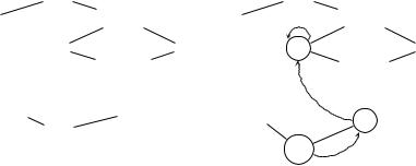
Fig. 12.4. (a) A complete lattice with (b) monotone function f

– s. s s = s.

Additionally, they satisfy the absorption laws:

•s1, s2. s1 (s1 s2) = s1;

•s1, s2. s1 (s1 s2) = s1.

One can define a partial order on S:

s1, s2. s1 s2 ↔ s1 = s1 s2 ,

or equivalently

s1, s2. s1 s2 ↔ s2 = s1 s2 .

A lattice is complete if for every subset S′ S (including infinite subsets), both the join, or supremum, S′ and the meet, or infimum, S′ exist. In particular, a complete lattice has a least element S and a greatest elementS. Figure 12.4(a) visualizes a complete lattice.

A function f on elements of a lattice is monotone in the lattice if

s1, s2. s1 s2 → f (s1) f (s2) .

A fixpoint of f is any element s S such that f (s) = s. The dashed lines of Figure 12.4(b) visualize the iterative application of monotone function f from S until it reaches the fixpoint s3.

The following theorem is an important classical result for monotone functions on complete lattices.

Theorem 12.18 (Knaster-Tarski Theorem). The fixpoints of a monotone function on a complete lattice comprise a complete lattice.

Since complete lattices are nonempty, a fixpoint of a monotone function on a complete lattice always exists. More, the Knaster-Tarski theorem guarantees the existence of the least fixpoint and the greatest fixpoint of f , which are the least and greatest elements, respectively, of the complete lattice defined by f ’s fixpoints.

Abstract Interpretation

An important complete lattice for our purposes is the lattice defined by the sets of a program P ’s possible states S: the join is set union, the meet is set intersection, and the partial order is set containment. The greatest element is the set of all states; the least element is the empty set. The lattice is thus represented by (2S , , ∩), where 2S is the powerset of S. Call this lattice CP .

Treat P as a function on S: P (s) is the successor state of s during execution. Define the strongest postcondition on subsets S′ of states S and program

P :

which we abbreviate as P (S′). Now define the function

FP is a monotone function on CP . Hence, by the Knaster-Tarski theorem, the least fixpoint of FP exists on CP : it is the set of reachable states of P . The lattice CP and the monotone function FP define the concrete semantics of program P . For this reason, the elements 2S of CP comprise the concrete domain.

The ForwardPropagate algorithm of Figure 12.2 can be described as applying FP to the set of states satisfying the function precondition until the least fixpoint is reached.

However, the least fixpoint of FP usually cannot be computed in practice (see Section 12.1.4). Therefore, consider another lattice, AP : (A, , ), whose elements A are “simpler” than those of CP . Its elements A might be intervals or a ne equations, for example, and thus comprise the abstract domain. Define two functions

α : 2S → A and γ : A → 2S ,

the abstraction function and the concretization function, respectively. These functions should preserve order:

S1, S2 S. S1 S2 → α(S1) α(S2) ,

and

a1, a2 A. a1 a2 → γ(a1) γ(a2) .

344 12 Invariant Generation

A monotone function F P on AP is a valid abstraction of FP if

a A. FP (γ(a)) γ(F P (a)) ,

that is, if the set of program states represented by abstract element F P (a) is a superset of the application of FP to the set of states represented by abstract element a. One possible abstraction is given by applying FP to the concretization of a and then abstracting the result:

def

F P (a) = α(FP (γ(a))) .

A valid abstraction F P provides a means for approximating the least fixpoint of FP in CP : the concretization γ(a) of any fixpoint a of F P in AP is a superset of the least fixpoint of FP in CP .

Lattice AP need not be any better behaved than CP , though. A wellbehaved lattice satisfies the ascending chain condition: every nondecreasing sequence of elements eventually converges. Consequently, computing the least fixpoint of a monotone function in such a lattice requires only a finite number of iterations. The lattice defined by the a ne spaces of Karr’s analysis trivially satisfies this condition: it is of finite height because the number of dimensions is finite. But, for example, the lattice defined by intervals does not satisfy the ascending chain condition. In this case, one must define a widening operator on the abstract domain.

Relating Notation and Concepts

In our presentation, we take as our concrete set not 2S but rather FOL representations of sets of states. The concrete lattice is thus (FOL, , ) with partial order . This lattice is not complete: there need not be a finite firstorder representation of the conjunction of an infinite number of formulae. But not surprisingly, there need not be a finite represention of a set of infinite cardinality, either, so the completeness of CP is not of practical value.

Our abstract domains are given by syntactic restrictions on the form of FOL formulae. The abstraction function is νD , and the concretization function is just the identity. spD is a valid abstraction of sp, and both are monotone in their respective lattices.

12.5 Summary

This chapter describes a methodology for developing algorithms to reason about program correctness. It covers:

•Invariant generation in a general setting. The forward propagation algorithm based on the strongest postcondition. The need for abstraction. Issues: decidability and convergence. Abstract interpretations.

Exercises 345

•Interval analysis, an abstract interpretation with a domain describing intervals. It is appropriate for reasoning about simple bounds on variables.

•Karr’s analysis, an abstract interpretation with a domain describing a ne spaces. It discovers equations among rational or real variables.

•Notation and concepts in the standard presentation of abstract interpretation.

This chapter provides just an introduction to a widely studied area of research.

Bibliographic Remarks

We present a simplified version of the abstract interpretation framework of Cousot and Cousot, who also describe a version of the interval domain that we present [20].

Karr developed his analysis a year before the abstract interpretation framework was presented [46]. For background on linear algebra, see [42]. Our presentation of Karr’s analysis is based on that of M¨uller-Olm and Seidl [63].

Many other domains of abstract interpretation have been studied. The most widely known is the domain of polyhedra, which Cousot and Halbwachs describe in [21]. Exercise 12.4 explores the octagon domain of Min´e [61]. As an example of a non-numerical domain, see the work of Sagiv, Reps, and Wilhelm on shape analysis [96].

Exercises

12.1 (wp and sp). Prove the second implication of Example 12.2; that is, prove that

Fwp(sp(F, S), S) .

12.2(General sp). Compute sp(F, ρ1) and sp(F, ρ2) for transition relations ρ1 and ρ2 of (12.1) and (12.2), respectively. Show that disregarding pc reveals the original definition of sp.

12.3(General wp and sp). For the general definitions of wp and sp, prove

that

sp(wp(F, S), S) F wp(sp(F, S), S) .

12.4 (Octagon Domain). Design an abstract interpretation for the octagon domain. That is, extend the interval domain to include literals of the form

c ≤ v1 + v2 , v1 + v2 ≤ c , c ≤ v1 − v2 , and v1 − v2 ≤ c .

Apply it to the loop of Example 12.4. Because i and n are integer variables, the loop guard i < n is equivalent to i ≤ n − 1.

346 12 Invariant Generation

12.5 (Non-a ne assignments). Consider a ne spaces F and

G : [[xk := 0]]F DK [[xk := 1]]F .

Prove the following:

(a)If [x1 · · · xk · · · xn] F , then [x1 · · · m · · · xn] G for all m R.

(b)If [x1 · · · xk · · · xn] G, then [x1 · · · m · · · xn] F for some m R.

Hint : Use the definition of the a ne hull.

12.6( Analyzing programs).

(a)Describe how to use AbstractForwardPropagate to analyze programs with many functions, some of which may be recursive. Hints: First, include a location in each function to collect information for the function postcondition. Consider that this information might include function variables other than rv and the parameters, so define an abstract operator elim to eliminate these variables. Then recall that function calls in basic paths are replaced by function summaries constructed from the function postconditions. Therefore, AbstractForwardPropagate need not be modified to handle function calls. But in which order should functions be analyzed? What about recursive functions?

(b)Describe an instance of this generalization for interval analysis. In particular, define elim.

(c)Describe an instance of this generalization for Karr’s analysis. In particular, define elim.

13

Further Reading

Do not seek to follow in the footsteps of the men of old; seek what they sought.

— Matsuo Basho

Kyoroku Ribetsu no Kotoba, 1693

In this book we have presented a classical method of specifying and verifying sequential programs (Chapters 5 and 6) based on first-order logic (Chapters 1–3) and induction (Chapter 4). We then focused on algorithms for automating the application of this method: decision procedures for reasoning about verification conditions (Chapters 7–11), and invariant generation procedures for deducing inductive facts about programs (Chapter 12). This material is fundamental to all modern research in verification. In this chapter, we indicate topics for further reading and research.

First-Order Logic

Other texts on first-order logic include [87, 31, 55]. Smullyan [87], on which the presentation of Section 2.7 is partly based, concisely presents the main results in first-order logic. Enderton [31] provides a comprehensive discussion of theories of arithmetic and G¨odel’s first incompleteness theorem. Manna and Waldinger [55] explore additional first-order theories.

Decision Procedures

We covered three forms of decision procedures: quantifier elimination (Chapter 7) for full theories, decision procedures for quantifier-free fragments of theories with equality (Chapters 8–10), and instantiation-based procedures for limited quantification (Chapter 11). New decision procedures in each of these styles are discovered regularly (see, for example, the proceedings of the

IEEE Symposium on Logic in Computer Science [51]).

348 13 Further Reading

Proofs of correctness in Chapters 7 and 11 appeal to the structure of interpretations. Model theory studies logic from the perspective of models (interpretations), and decision procedures can be understood in model-theoretic terms. Hodges covers this topic comprehensively [40].

The combination result of Chapter 10 is not the only one known, although it is the simplest general result. For example, Shostak’s method treats a subclass of fragments with greater speed [84, 78]. Current e orts aim to extend combination methods to require fewer or di erent restrictions [93, 99, 94, 4]. However, most theories cannot be combined in a general way, particularly when quantification is allowed, so logicians develop special combination procedures [100].

Decision procedures for PL (“SAT solvers”) and combination procedures (“SMT”, for SAT Modulo Theories) have received much practical attention recently, even in the form of annual competitions [81, 86]. Motivating applications include software and hardware verification.

Automated Theorem Proving

While satisfiability/validity decision procedures have obvious advantages — speed; the guarantee of an answer in theory and often in practice; and, typically, the ability to produce counterexamples — not all theories or interesting fragments are decidable. For example, reasoning about permutations of arrays is undecidable in certain contexts (see Exercise 6.5 and [77, 6]), yet we would like to prove, for example, that sorting functions return permutations of their input.

Because FOL is complete, semi-decision procedures (see Section 2.6.2) are possible: the procedure described before the proof of Lemma 2.31 is such a procedure. More relevant are widely-used procedures with tactics [76, 67, 47]. Recent work has looked at e ectively incorporating decision procedures into general theorem proving [48]. The specification language for verified programming is more expressive using these procedures. However, proving verification conditions sometimes requires user intervention.

FOL may not be su ciently expressive for some applications. Second-order logic extends first-order logic with quantification over predicates. Despite being incomplete, researchers continue to investigate heuristics for partly automating second-order reasoning [67]. Separation logic is another incomplete logic designed for reasoning about mutable data structures [75].

Static Analysis

Static analysis is one of the most active areas of research in verification. Classically, static analyses of the form presented in Chapter 12 have been studied in two areas: compiler development and research [62] and verification [20].

Important areas of current research include fast numerical analyses for discovering numerical relations among program variables [80], precise alias

and shape analyses for discovering how a program manipulates memory [96], and predicate abstraction and refinement [5, 37, 16, 24].

Static analyses of the form in Chapter 12 solve a set of implications for a fixpoint (an inductive assertion map is a fixpoint) by forward propagation. Other methods exist for finding fixpoints, including constraint-based static analysis [2, 17].

Static analyses also address total correctness by proving that loops and functions halt [18, 7, 8]. Their structure is di erent than the analyses of Chapter 12 as they seek ranking functions.

Concurrent Programs

We focus on specifying and verifying sequential programs in this book. Just as concurrent programs are more complex than sequential programs, specification and verification methodologies for concurrent programs are more complex than for sequential programs. Fortunately, many of the same methods, including the inductive assertion method and the ranking function method, are still of fundamental importance in concurrent programming. Manna and Pnueli provide a comprehensive introduction to this topic [53, 54]. Milner describes a calculus of concurrent systems in which both the system and its specification is written [60].

Temporal Logic

Because functions of pi do not have side e ects, specifying function behavior through function preconditions and postconditions is su cient. However, reactive and concurrent systems, such as operating systems, web servers, and computer processors, exhibit remarkably complex behavior. Temporal logics are typically used for specifying their behavior.

A temporal logic extends PL or FOL with temporal operators that express behavior over time. Canonical behaviors include invariance, in which some condition always holds; progress, in which a particular event eventually occurs; and reactivity, in which a condition causes a particular event to occur eventually.

Temporal logics are divided into logics over linear-time structures (Linear Temporal Logic (LTL)) [53]; branching-time structures (Computational Tree Logic (CTL), CTL ) [14]; and alternating-time structures (Alternating-time Temporal Logic (ATL), ATL ) [3].

Model Checking

A finite-state model checker [15, 74] is an algorithm that checks whether finitestate systems such as hardware circuits satisfy given temporal properties.

An explicit-state model checker manipulates sets of actual states as vectors of bits. A symbolic model checker uses a formulaic representation to represent

350 13 Further Reading

sets of states, just as we use FOL to represent possibly infinite sets of states in Chapters 5 and 6. The first symbolic model checker was for CTL [12]; it represents sets of states with Reduced Ordered Binary Decision Diagrams (ROBDDs, or just BDDs) [10, 11].

LTL model checking is based on manipulating automata over infinite strings [95]. A rich literature exists on such automata; see [91] for an introduction.

Predicate abstraction and refinement [5, 37, 16, 24] has allowed model checkers to be applied to software and represents one of the many intersections between areas of research (model checking and static analysis in this case).

Clarke, Grumberg, and Peled discuss model checking in detail [14].