

Bradley, Manna. The Calculus of Computation, Springer, 2007
.pdf230 |
8 |
Quantifier-Free Linear Arithmetic |
|||||||
A2 |
= |
−2 1 |
|
and |
b2 |
= |
|
2 |
. |
|
|
1 0 |
|
|
|
|
|
0 |
|
In Figure 8.4, the rows of A2 and b2 correspond to the vertical and diagonal constraints, respectively, which are the defining constraints of v2.
In the next iteration, solving A |
Tu = c yields u |
|
= |
3 1 |
|
T. Adding 0s for |
|||
rows not in R produces |
2 |
2 |
2 |
|
|
|
|||
u = |
3 0 1 |
T . |
|
|
|
|
|
|
|
Since u ≥ 0, we are in Case 1. The maximum is |
|
|
|
|
|
||||
cTv2 = −1 1 2 |
= 2 |
|
|
|
|
|
|
||
|
|
0 |
|
|
|
|
|
|
|
at vertex v2. |
|
|
|
|
|
|
|
|
|
This move from vertex vi to vertex vi+1 makes progress. For
cTvi+1 = cT(vi + λiy)
=cTvi + λicTy
=cTvi + λi(−uk) > cTvi .
When considering line 3, recall from (8.5) of the construction of u that
uiT = cTA−i 1
and that the k′th column of A−i 1 is −y by (8.8). Hence, cTy = −uk. Moreover, since there are only a finite number of vertices to examine, Case
1 (or, in the general case, possibly Case 2(b)) eventually occurs.
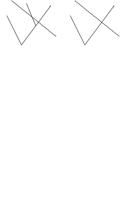
Figure 8.5(a) illustrates this case: vertex vi+1 is discovered by moving along ray y as far as possible without violating the constraints. Moreover
cTvi+1 is greater than cTvi.
It is possible that λi = 0 when the vertex vi has multiple sets of defining constraints. However, because there are only a finite number of constraints, the number of defining constraint sets is also finite. Preventing repetitions of the matrix Ai across iterations guarantees that the algorithm still halts in this case.
Case 2(b): Optimum is Unbounded
In this case, Ay ≤ 0 and the optimum is unbounded. Since Ay ≤ 0, for all λ ≥ 0,
A(vi + λy) = Avi |
+λ Ay |
≤ |
b , |
|{z} |
|{z} |
|
|
≤b |
≤0 |
|
|
8.4 The Simplex Method |
231 |
vi+1 • |
|
|
|
Ax ≤ b |
cTx |
Ax ≤ b |
cTx |
y |
|
y |
|
• |
|
• |
|
vi |
|
vi |
|
(a) |
|
(b) |
|
Fig. 8.5. Case 2
so all vi + λy satisfy the constraints. In other words, moving in direction y either moves along the boundary of a constraint (ay = 0) or moves inward (ay < 0). Moreover,
cT(vi + λy) = cTvi + λcTy |
|
|
|
|
|
|
= cTvi + λuTAy |
|
|
|
|
|
|
= cTvi + −λ uk |
, |
|
|
|
|
|
|{z}T |
|
T |
|
|
T |
|
<0 |
|
|
|
|
|
|
which grows with λ (recall c = u A, and Ay = 0 · · · 0 −1 0 · · · 0 |
|
|
by |
|||
selection of y). Thus, the maximum is unbounded. Figure 8.5(b) |
illustrates |
|||||
|
|
|
|
|||
this case: all points along the ray labeled y satisfy the constraints, and moving along the ray increases cTx without bound.
Example 8.15. Continuing with y = |
1 0 0 0 0 |
|
T |
from Example 8.13, com- |
|||||||||||||
pute Ay |
|
|
|
|
0 |
|
|
|
|
|
|
|
|
|
|||
−0 1 |
0 |
0 |
|
1 |
|
|
−0 |
|
|
|
|||||||
|
1 |
|
0 |
0 |
0 |
0 |
|
|
|
|
|
|
1 |
|
|
|
|
|
0 |
−0 |
1 |
0 |
0 |
|
0 |
= |
|
0 |
|
|
|
|
|||
0 |
|
0 |
−0 |
1 |
0 |
|
0 |
|
0 |
|
|
|
|||||
|
0 |
|
0 |
0 |
−0 |
1 |
|
|
0 |
|
|
|
0 |
|
|
|
|
|
|
|
|
|
|
|
|
|
|||||||||
|
1 |
|
1 |
1 |
1 |
−0 |
|
|
0 |
|
|
|
1 |
|
|
|
|
|
|
|
|
|
|
|
|
|
|
|
|||||||
|
|
|
|
|
|
|
|
|
|
|
|
|
|
|
|
|
|
|
−1 1 |
1 |
−1 |
1 |
|
|
|
|
|
|
−1 |
|
|
|
|
||
|
|
− |
|
A |
|
|
|
|
y |
|
|
|
|
|
|
|
|
|
|
|
− − |
| {z } |
|
|
|
|
|
|
|
||||||
| {z } |
|
|
|
|
|
|
|
|
|
|
|||||||
to find that S = [7] since a7y = 1 > 0. Thus, according to (8.10), examine the seventh row of the constraints and choose the greatest λ1 such that

232 |
8 Quantifier-Free Linear Arithmetic |
|
|
|
|
|
|
|
|
|
|
|||||
|
|
|
|
|
|
|
|
|
0 |
|
0 |
|
||||
|
|
|
|
|
|
|
|
|
|
0 |
|
|
|
1 |
|
|
|
1 −1 1 −1 −1 |
|
(v1 |
+ λ1y) = |
|
− − − |
|
|
0 |
|
+ λ1 |
|
0 |
|
= 1 ; |
|
a7 |
|
|
|
|
|
|
0 |
|
|
|
0 |
|
|
|||
|
|
|
|
|
1 |
1 1 |
1 |
1 |
|
|
|
|
|
|
||
| {z } |
|
|
|
|
|
|
|
|
|
|
|
|
|
|
||
|
|
|
|
|
|
|
|
|
|
|
|
|
|
|||
that is, choose λ1 = 1. By (8.12), define v2 = v1 + λ1y = 1 0 0 0 0 T .
Form A2 by replacing the first row (k′ = 1) of A1 with the seventh row (ℓ = 7) of A:
|
|
|
0 −1 |
0 |
|
0 |
0 |
|
|
|
|
|
1 |
−1 |
1 |
−1 |
−1 |
. |
|
A2 |
= |
0 |
0 −0 |
|
1 |
0 |
|||
|
|
|
|
|
|
− |
|
|
|
|
|
|
0 |
0 |
1 |
0 |
0 |
|
|
|
|
|
|
|
|
|
|
|
|
|
|
|
|
|
|
|
|
|
|
00 0 0 −1
This move to vertex v2 makes progress:
cTv1 = 0 < cTv2 = 1 .
Now R = [7; 2; 3; 4; 5]; that is, A2 is the submatrix of A constructed from rows 7, 2, 3, 4, and 5. Solve A2Tu2 = c for u2, yielding u2 = [1 0 0 0 0]T. Since u2 ≥ 0, we are in Case 1: we have found an optimum point v2 with optimal value 1.
Recall from Example 8.7 that vG = 1Tg2 = 1. The equality of the optimum and vG implies that
F : x + y ≥ 1 x − y ≥ −1
is TQ-satisfiable. In particular, extract from
x2 |
|
|
|
|
0 |
|
|
|
x1 |
|
|
|
|
1 |
|
y1 |
|
= v2 |
= |
0 |
|||
|
2 |
|
|
|
|
0 |
|
|
z |
|
|
|
|
|
|
|
y |
|
|
|
|
0 |
|
|
|
|
|
|
|
|
|
the assignment |
|
x = x1 − x2 = 1 − 0 = 1 |
and y = y1 − y2 = 0 − 0 = 0 , |
which indeed satisfies F . |
|
Example 8.16. Consider the ΣQ-formula
F : x ≥ 0 y ≥ 0 x ≥ 2 y ≥ 2 x + y ≤ 3 ,

8.4 The Simplex Method |
233 |
or, in matrix form, |
|
|
|
|||||
|
−0 −1 |
|
x |
0 |
||||
|
|
1 |
0 |
|
y ≤ |
|
0 |
. |
F : |
−0 |
1 |
−2 |
|||||
|
|
1 |
−1 |
|
|
|
−3 |
|
|
|
|
|
|
|
|||
|
|
1 |
0 |
|
|
|
2 |
|
|
|
|
|
|
|
|
|
|
Is F TQ-satisfiable? Because F has only weak inequality literals, the corresponding linear program has a constant objective function:
M : max 1 |
|
|
|
|
|
|
|
|
|
subject to |
|
|
|
x |
|
|
0 |
|
|
|
−0 −1 |
|
|||||||
|
|
1 |
0 |
|
y |
≤ |
|
0 |
|
G : |
−0 |
1 |
−2 |
||||||
|
|
1 |
−1 |
|
|
|
|
−3 |
|
|
|
|
|
|
|
|
|||
|
|
1 |
0 |
|
|
|
|
2 |
|
|
|
|
|
|
|
|
|
|
|
Solving the corresponding linear program M0 is su cient to determine the TQ-satisfiability of F .
Construction of M0
Because x and y are already constrained to be nonnegative, we do not need to introduce new x1, x2, y1, y2. Rewrite the final three literals of F as two sets
of constraints: |
|
|
|
|
|
|
|
|
|
|
|
x |
≤ |
|
|
1 0 |
x |
≥ |
|
2 |
|||
[1 1] y |
[3] |
and |
0 1 |
y |
2 |
||||||
D1 |
|
g1 |
|
| {z } |
|
|
|{z} |
||||
|{z} |
|
|{z} |
|
|
|
||||||
|
|
|
|
|
D2 |
|
|
|
|
g2 |
|
|
|
|
|
|
|
|
x |
|
|
|
|
|
|
|
|||
M0 : max [1 1 |
1 |
|
1] |
|
|
y |
|
|
|
|
|
|
|
||||
|
|
|
z |
|
|
|
|
|
|
|
|||||||
|
|
−cT |
− |
|
|
|
|
|
|
|
|
|
|
|
|||
|
|
|
|
z1 |
|
|
|
|
|
|
|||||||
subject to |
|
|
|
|
2 |
|
|
|
|
|
|
|
|||||
|
|
|
|
|
|
|
|
|
|
|
|
|
|||||
| |
|
{z } |
|
|
|
|
|
|
|
|
|
|
|
|
|||
|
1 |
0 |
0 |
|
|
0 |
|
|
|
|
|
|
0 |
||||
−0 −1 |
0 |
|
|
0 |
|
|
x |
|
|
0 |
|||||||
|
0 |
0 |
1 |
|
|
0 |
|
y |
|
|
0 |
|
|||||
0 |
0 |
−0 1 |
|
0 |
|||||||||||||
|
1 |
1 |
0 −0 |
|
|
|
z |
1 |
|
≤ |
|
3 |
|
||||
|
|
z |
|
|
|
||||||||||||
|
1 |
0 |
1 |
|
|
0 |
|
2 |
|
|
2 |
|
|||||
|
|
|
|
|
|
|
|
|
|
||||||||
|
0 |
1 |
−0 |
|
|
1 |
|
|
|
|
|
|
|
2 |
|
||
|
|
|
|
|
|
|
|
|
|
|
|
||||||
|
|
|
|
|
|
|
|
|
|
|
|
|
|
|
|
|
|
|
|
|
|
|
− |
|
|
|
|
|
|
|
|
|
|
|
|
| {z } |
|
|
|
|
|
|
| {z } |
||||||||||
A |
b |
|

234 8 Quantifier-Free Linear Arithmetic |
|
|
|
|
|
|
|||||||
in which c is computed according to |
|
|
|
|
y |
|
|||||||
cTx = 1T D2 |
|
I |
y |
|
= [1 1] |
1 0 |
1 |
|
0 |
||||
|
|
|
|
x |
|
|
|
|
1 |
|
x |
||
|
− |
|
|
z1 |
|
0 1 |
−0 |
− |
|
z1 |
|
||
|
|
z2 |
|
|
|
|
z2 |
||||||
|
|
|
|
|
|
|
|
|
|
|
|
|
|
|
|
|
|
|
|
|
|
|
|
|
|
|
|
= 1 1 1 1 |
y |
. |
|
cT |
|
x |
|
z2 |
|
||
− − |
|
|
|
| {z } |
|
|
|
Use the initial vertex
x0
|
|
z1 |
|
|
|
0 |
|
|
v1 |
= |
|
y |
|
= |
|
0 |
|
2 |
|
|||||||
|
|
|
z |
|
|
|
0 |
|
|
|
|
|
|
|
|
||
to start the vertex traversal.
F is satisfiable i the optimal value is equal to
vG = 1 |
|
g2 |
= [1 1] |
2 |
= 4 . |
|
T |
|
|
2 |
|
We apply the simplex method to find the optimum.
Iteration 1
Choose rows R = [1; 2; 3; 4] of A and b to form
A1 |
= |
−0 |
−1 |
0 |
|
0 |
|
and b1 = |
0 |
. |
|
|
|
|
1 |
0 |
0 |
|
0 |
|
|
0 |
|
|
|
0 |
0 |
−0 |
|
1 |
0 |
||||
|
|
|
|
|
|
− |
|
|
|
|
|
|
|
|
0 |
0 |
1 |
|
|
0 |
|
||
|
|
|
|
0 |
|
|
|
||||
This submatrix and subvector correspond to the defining constraints of vertex
v1: A1v1 = b1. |
|
|
|
|
|
|
|
|
|
||||||||
|
|
|
Recall that by the Duality Theorem (Theorem 8.6), our goal is to find a |
||||||||||||||
vector u such that u |
≥ |
0 and uTA = cT. We use A |
to solve for a u satisfying |
||||||||||||||
u |
T |
A = c |
T |
|
|
|
|
|
|
|
1 |
|
|
||||
|
|
and, through iteratively exploring a sequence of vertices, eventually |
|||||||||||||||
find a u that also satisfies u ≥ 0. |
T |
|
|||||||||||||||
|
|
|
Therefore, |
we |
solve |
for u. By (8.5), solve A1 |
|
u1 = c to yield u1 = |
|||||||||
|
|
1 |
|
1 1 1 |
T. Adding 0s for the rows not in R produces u: |
||||||||||||
− |
|
− |
|
|
|
|
1 1 0 0 0 |
|
T |
|
|
|
|||||
|
|
|
u = −1 −1 T |
A = c |
T |
|
, |
|
|
||||||||
which satisfies u |
|
(8.6) as desired. |
|
|
|||||||||||||

8.4 The Simplex Method |
235 |
Since u1, u2 < 0, we are in Case 2 with k = k′ = 1. We have not yet found a u ≥ 0, so we must continue searching. In particular, constraints 1 and 2 are causing a problem (as indicated by u1, u2 < 0), so we must find a direction y and distance λ1 to travel to a better vertex whose defining constraints do not
include constraint 1. The direction is given by the first column of −A−1: by (8.8), solve A1y = −e1 to yield y = 1 0 0 0 T. 1
It remains to find the distance λ1 to travel along y. Computing Ay shows that S = [5; 6]: the fifth and sixth rows a of A are such that ay > 0. This situation means that traveling along y too far will result in making one or both of constraints 5 and 6 unsatisfied. The other constraints will continue to be satisfied independent of λ1.
Therefore, by (8.9), choose the largest λ1 such that
A(v1 + λ1y) ≤ b .
Focusing on the fifth and sixth rows of A (since S = [5; 6]), choose the largest λ1 such that
|
|
|
|
0 |
|
+ λ1 |
1 |
|
|
|
1 1 |
|
0 0 |
|
0 |
0 |
|
≤ |
3 |
||
1 0 |
− |
1 0 |
|
0 |
|
|
0 |
|
2 |
|
|
|
|
0 |
|
|
0 |
|
|
|
|
|
|
|
|
|
|
|
||||
|
|
|
|
|
|
|
y |
|
|
|
| {z } |
v1 |
|
|
|
|
|{z} |
||||
| {z } |
| {z } |
|
||||||||
rows 5,6 of A |
|
|
|
|
|
|
|
rows 5,6 of b |
||
according to (8.9). Namely, choose λ1 = 2 (and ℓ = 6).
We now have a direction (y) and a distance (λ1) to travel away from v1.
By (8.12), define |
|
|
|
0 |
= 0 . |
||||
v2 = v1 + λ1y = 0 |
+ 2 |
||||||||
|
0 |
|
|
|
1 |
|
|
2 |
|
0 |
|
0 |
0 |
||||||
|
|
|
|
|
|
|
|
|
|
|
0 |
|
|
|
0 |
|
|
0 |
|
|
|
|
|
|
|
|
|||
For the next iteration, replace the first row of A1 (since k′ = 1) with the sixth row of A (since ℓ = 6) to produce
A2 = |
0 −1 |
−0 |
|
0 |
|
and b2 = |
0 |
. |
|
|
1 |
0 |
1 |
|
0 |
|
|
2 |
|
0 |
0 |
−0 |
|
1 |
0 |
||||
|
|
|
|
− |
|
|
|
|
|
|
0 |
0 |
1 |
0 |
|
|
0 |
|
|
|
|
|
|
|
|||||
Have we made progress by moving to vertex v2? Yes, for
cTv1 = 0 < 2 = cTv2 .
The objective function has increased from 0 to 2.

236 |
8 Quantifier-Free Linear Arithmetic |
|
|
Iteration 2 |
|
|
|
Now R = [6; 2; 3; 4]. Solve A2Tu2 = c to yield u2 |
= 1 −1 0 1 |
T for rows |
|
[6; 2; 3; 4]. Then filling in 0s for the other rows of A |
produces: |
|
|
|
|||
u = [0 −1 0 1 0 1 0]T . row: 2 3 4 6
Note that u maintains the order of rows, while u2 is ordered according to R. u2 < 0, so k = 2, which corresponds to row k′ = 2 of u2. According to Case 2, let y be the second column of −A−2 1: solve A2y = −e2 to yield y = [0 1 0 0]T. Then the fifth and seventh rows a of A are such that ay > 0 so that S = [5; 7]. Focusing on the fifth and seventh rows of A, choose the largest λ2 such that
|
|
|
|
2 |
|
+ λ2 |
0 |
|
|
|
|
1 1 0 |
|
0 |
|
0 |
1 |
|
≤ |
3 |
. |
||
0 1 0 |
− |
1 |
|
0 |
|
|
0 |
|
2 |
|
|
|
|
|
0 |
|
|
0 |
|
|
|
|
|
|
|
|
|
|
|
|
|
||||
|
|
|
|
|
|
|
|
|
|
|
|
| {z } |
v2 |
|
|
b |
|
|
|{z} |
||||
| {z } |
| {z } |
|
|||||||||
rows 5,7 of A |
|
|
|
|
|
|
|
rows 5,7 of b |
|||
Choose λ2 = 1 (and ℓ = 5). Then
v3 = v2 + λ2y = 0 |
+ 1 |
1 |
= 1 . |
||||||
|
2 |
|
|
|
0 |
|
|
2 |
|
0 |
|
0 |
0 |
||||||
|
|
|
|
|
|
|
|
|
|
|
0 |
|
|
|
0 |
|
|
0 |
|
|
|
|
|
|
|
|
|||
Replace the second row of A2 (since k′ = 2) with the fifth row of A (since ℓ = 5) to produce
A3 = |
1 1 |
−0 |
|
0 |
|
and b3 = |
3 |
. |
|
1 0 |
1 |
|
0 |
|
|
2 |
|
0 0 |
−0 |
|
1 |
0 |
||||
|
|
|
− |
|
|
|
|
|
|
0 0 |
1 |
0 |
|
|
0 |
|
|
|
|
|
|
|
Have we made progress? Yes, for
cTv1 = 0 < cTv2 = 2 < cTv3 = 3 .
The objective function has increased from 2 to 3.
Iteration 3 |
|
|
|
|
|||
Now R = [6; 5; 3; 4]. Solve A3Tu3 = c, yielding u3 = |
0 1 1 1 |
T. Because |
|||||
u |
3 |
≥ |
0, we are in Case 1: v |
3 |
is the optimum with objective value |
||
|
|
|
|
|
|||

|
|
1 |
8.5 Summary 237 |
||
cTv3 = 1 1 1 1 |
= 3 . |
||||
|
− − |
|
2 |
|
|
0 |
|
||||
|
|
|
|
|
|
|
|
|
0 |
|
|
|
|
|
|
|
|
The optimal value of the constructed optimization problem is 3, which is less than the required vG = 4. The constraints G of the linear program M are unsatisfiable, and thus F itself is TQ-unsatisfiable.
8.4.3 Complexity
Theorem 8.17. TQ-satisfiability of conjunctive quantifier-free ΣQ-formulae is weakly polynomial-time decidable.
An algorithm is weakly polynomial-time if it runs in time polynomial in the actual values of the input, not just the size of the input. Bibliographic Remarks discusses algorithms that achieve this performance.
While e cient in practice, the simplex method actually has poor worstcase behavior for known fixed pivot rules. A pivot rule determines which adjacent vertex to visit next. In our presentation, no rule is fixed: the next vertex can be any of those corresponding to the negative entries in the u vector. However, for all known pivot rules, there exist classes of quantifier-free ΣQ-formulae on which the simplex method requires an exponential number of steps in the size of the formulae.
8.5 Summary
This chapter covers linear programming and the simplex method for solving linear programs. It covers:
•How decision procedures that reason only about conjunctive formulae extend to arbitrary Boolean structure by converting to DNF. Exercise 8.1 explores a more e ective way of converting to DNF.
•A review of linear algebra.
•Linear programs, which are optimization problems with linear constraints and linear objective functions. Application to TQ-satisfiability.
•The simplex method. Finding an initial point via a new linear program. Greedy search along vertices.
The structure of the simplex method is markedly di erent from the structure of the quantifier elimination procedures of Chapter 7. It focuses on the structure of the set of interpretations of the given formula, rather than on the formula itself. Exercises 8.3, 8.4, and 8.5 explore these sets, which describe polyhedra.
238 8 Quantifier-Free Linear Arithmetic
In addition to applications in all of engineering, arithmetical reasoning is necessary for analyzing program correctness. Of course, arithmetic usually appears in the context of other data structures in software. Chapter 10 discusses a method for combining the arithmetic decision procedures of this and the previous chapter with other decision procedures.
Bibliographic Remarks
For a presentation of linear algebra, see [42]; for a comprehensive presentation of linear and integer programming, see [82].
Work on linear programming proceeded in parallel in the western hemisphere and the USSR. Dantzig is the inventor of the simplex method in the western hemisphere [22]. Earlier work by Kantorovich in the USSR also proposes the method [44]. Weakly polynomial-time algorithms were achieved by Khachian [49] in the USSR and Karmarkar [45] in the western hemisphere.
Exercises
8.1 ( Conjunctive quantifier-free formulae). Converting an arbitrary quantifier-free Σ-formula to DNF and then applying a decision procedure to each disjunct can be prohibitively expensive. In practice, SAT solvers (decision procedures for propositional logic, such as DPLL) are used to extend a decision procedure for conjunctive quantifier-free Σ-formula to arbitrary quantifier-free Σ-formula.
(a) Show that the DNF of a formula F can be exponentially larger than F . (b) Describe a procedure that, using a SAT solver, extracts conjunctive Σ-
formulae from a quantifier-free Σ-formula F . Using this procedure, each discovered conjunctive formula’s T -satisfiability will be decided. If it is T -satisfiable, then F is T -satisfiable, so the procedure finishes; otherwise, the procedure finds another conjunctive formula.
(c) The proposed procedure is really no more e cient than simply converting to DNF. This part explores an optimization. An unsatisfiable core of T - unsatisfiable conjunctive Σ-formula G is the conjunction H of a subset of literals of G such (1) H is also T -unsatisfiable, and (2) the conjunction of each strict subset of literals of H is T -satisfiable. Improve your procedure from the previous part to use a function UnsatCoreT (G) that returns a T -unsatisfiable core of a T -unsatisfiable conjunctive Σ-formula G.
(d) Given a decision procedure DPT for conjunctive quantifier-free Σ-formula, describe a procedure UnsatCore(G) for computing an unsatisfiable core of G that takes no more than a number of DPT calls linear in the number of literals of G. Note that G can have multiple unsatisfiable cores; your procedure need only return one.

Exercises 239
(e) Given a decision procedure DPT for conjunctive quantifier-free Σ-formula, describe a procedure UnsatCore(G) for computing an unsatisfiable core of G that takes no more than O(m log n) calls of DPT , where m is the number of literals of the returned unsatisfiable core and n is the number of literals of G.
8.2 (DP for TQ). Apply the simplex method to decide the TQ-satisfiability of the following ΣQ-formulae.
(a) x ≥ 1 2x ≤ 1
(b) x + 2y ≥ 1 2x + y ≥ 1 2x + 2y ≤ 1 (c) x + 2y ≥ 1 2x + y ≥ 1 x + y ≤ 1
8.3 ( Polyhedra & dual representation). Ax ≤ b defines a subspace of Rn called a polyhedron; Ax ≤ b is the constraint representation of this space. A polyhedron can also be described by the union of a set of vertices V Rn and a set of rays R Rn; this representation is the vertex representation. While vertices v V describe points in Rn, rays r R describe directions in Rn. For example, as a vertex, [1 1]T R2 describes the point one unit right and one unit up from the origin on the plane. As a ray, it describes the “northeast” direction.
Represent each vertex v V and ray r R by the (n + 1)-vectors
|
1 |
|
and |
|
0 |
|
, |
|
x |
|
|
|
r |
|
|
respectively. Let P be the union of V and R represented in this way. Then for every inequality Ax ≤ b, there exists a vertex-ray set P with k elements such that
Ax ≤ b i λ1, . . . , λk ≥ 0. |
1 |
= i=1 λipi . |
|
|
k |
|
x |
X |
|
|
|
(a) Given an element |
|
|
x |
|
|
p = ǫ P , |
|
|
we can evaluate Ax ≤ ǫb. If p is a vertex, it is equivalent to evaluating Ax ≤ b, as expected. If p is a ray, it is equivalent to evaluating Ax ≤ 0. Explain what the ray case means.
(b) Define the convex hull as follows:
hull(P ) = (x : λ1, . . . , λk ≥ 0. |
1 |
= |
λipi) . |
|
|
|
k |
x |
X |
||
|
|||
|
i=1 |
Show that hull(P ) is convex. Conclude that if Ax ≤ ǫb for each [xT ǫ]T P , then hull(P ) {x : Ax ≤ b}.