Bradley, Manna. The Calculus of Computation, Springer, 2007

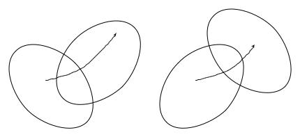
Fig. 12.1. (a) Weakest precondition and (b) strongest postcondition

forward propagation procedure for discovering inductive assertions. In general, this procedure is not an algorithm: it can run forever without producing an answer. Hence, Section 12.1.4 presents a methodology for constructing abstract interpretations of programs, which focus on particular elements of programs and apply a heuristic to guarantee termination. Subsequent sections examine particular instances of this methodology.

12.1.1 Weakest Precondition and Strongest Postcondition

Recall from Section 5.2.4 that a predicate transformer p is a function

p : FOL × stmts → FOL

that maps a FOL formula F FOL and program statement S stmts to a FOL formula. The weakest precondition predicate transformer wp(F, S) is defined on the two types of program statements that occur in basic paths:

• wp(F, assume c) c → F , and

•wp(F [v], v := e) F [e];

and inductively on sequences of statements S1; . . . ; Sn:

wp(F, S1; . . . ; Sn) wp(wp(F, Sn), S1; . . . ; Sn−1) .

The weakest precondition wp(F, S) has the defining characteristic that if state s is such that

s |= wp(F, S)

and if statement S is executed on state s to produce state s′, then

s′ |= F .

In other words, the weakest precondition moves a formula backward over a sequence of statements: for F to hold after executing S1; . . . ; Sn, the formula wp(F, S1; . . . ; Sn) must hold before executing the statements.

This situation is visualized in Figure 12.1(a). The region labeled F is the set of states that satisfy F ; similarly, the region labeled wp(F, S) is the set of states that satisfy wp(F, S). Every state s on which executing statement S leads to a state s′ in the F region must be in the wp(F, S) region.

For reasoning in the opposite direction, we define the strongest postcondition predicate transformer. The strongest postcondition sp(F, s) has the defining characteristic that if s is the current state and

s |= sp(F, S)

then there exists a state s0 such that executing S on s0 results in state s and

s0 |= F .

Figure 12.1(b) visualizes this characteristic. Executing statement S on any state s0 in the F region must result in a state s in the sp(F, S) region.

Define sp(F, S) as follows. On assume statements,

sp(F, assume c) c F ,

for if program control makes it past the statement, then c must hold.

Unlike in the case of wp, there is no simple definition of sp on assignments:

sp(F [v], v := e[v]) v0. v = e[v0] F [v0] .

Let s0 and s be the states before and after executing the assignment, respectively. v0 represents the value of v in state s0. Every variable other than v maintains its value from s0 in s. Then v = e[v0] asserts that the value of v in state s is equal to the value of e in state s0. F [v0] asserts that s0 |= F . Overall, sp(F, v := e) describes the states that can be obtained by executing v := e from F -states, states that satisfy F .

Finally, define sp inductively on a sequence of statements S1; . . . ; Sn:

sp(F, S1; . . . ; Sn) sp(sp(F, S1), S2; . . . ; Sn) .

sp progresses forward through the statements.

Example 12.1. Compute

sp(i ≥ n, i := i + k)

i0. i = i0 + k i0 ≥ n

i − k ≥ n

since i0 = i − k.

314 12 Invariant Generation

Compute

sp(i ≥ n, assume k ≥ 0; i := i + k)

sp(sp(i ≥ n, assume k ≥ 0), i := i + k)

sp(k ≥ 0 i ≥ n, i := i + k)

i0. i = i0 + k k ≥ 0 i0 ≥ n

k ≥ 0 i − k ≥ n

Example 12.2. Let us prove that

sp(wp(F, S), S) F wp(sp(F, S), S) ;

that is, the strongest postcondition of the weakest precondition of F on statement S implies F , which implies the weakest precondition of the strongest postcondition of F on S. We prove the first implication and leave the second implication as Exercise 12.1.

Suppose that S is the statement assume c. Then

sp(wp(F, assume c), assume c)

sp(c → F, assume c)

c (c → F )

c F

F

Now suppose that S is an assignment statement v := e. Then

sp(wp(F [v], v := e[v]), v := e[v])

sp(F [e[v]], v := e[v])

v0. v = e[v0] F [e[v0]]

v0. v = e[v0] F [v]

F

Recall the definition of a verification condition in terms of wp:

{F }S1; . . . ; Sn{G} : F wp(G, S1; . . . ; Sn) .

We can similarly define a verification condition in terms of sp:

{F }S1; . . . ; Sn{G} : sp(F, S1; . . . ; Sn) G .

Typically, we prefer working with the weakest precondition because of its syntactic handling of assignment statements. However, in the remainder of this chapter, we shall see the value of the strongest postcondition.

12.1.2 General Definitions of wp and sp

Section 12.1.1 defines the wp and sp predicate transformers for our simple language of assumption (assume c) and assignment (v := e) statements. This section defines these predicate transformers more generally.

Describe program statements with FOL formulae over the program variables x, the program counter pc, and the primed variables x′ and pc′. The program counter ranges over the locations of the program. The primed variables represent the values of the corresponding unprimed variables in the next state. For example, the statement

Li : assume c;

Lj :

is captured by the relation

To execute this statement, the program counter must be Li and c must be true. Executing the statement sets the program counter to Lj and leaves the variables x unchanged. Similarly, the assignment

Li : xi := e;

Lj :

is captured by the relation

ρ2[pc, x, pc′, x′] : pc = Li pc′ = Lj x′i = e pres(x \ {xi}) , (12.2)

where pres(V ), for a set of variables V , abbreviates the assertion that each variable in V remains unchanged:

^

v′ = v .

v V

Formulae (12.1) and (12.2) are called transition relations. The expressiveness of FOL allows many more constructs to be encoded as transition relations than can be encoded in either pi or the simple language of assumptions and assignments.

Let us consider the weakest precondition and the strongest postcondition in this general context. For convenience, let y be all the variables of the program including the program counter pc. The weakest precondition of F over transition relation ρ[y, y′] is given by

wp(F, ρ[y, y′]) y′. ρ[y, y′] → F [y′] .

Notice that free(wp(F, ρ)) = y. A satisfying y represents a state from which all ρ-successors, which are states y′ that ρ relates to y, are F -states. Technically,

316 12 Invariant Generation

such a state might not have any successors at all; for example, ρ could describe a guard that is false in the state described by y.

Consider the transition relation (12.1) corresponding to assume c:

wp(F, pc = Li pc′ = Lj c x′ = x)

pc′, x′. pc = Li pc′ = Lj c x′ = x → F [pc′, x′]pc = Li c → F [Lj , x]

Disregarding the program counter, we have recaptured our original definition of wp on assume statements:

wp(F, assume c) c → F .

Similarly,

wp(F, pc = Li pc′ = Lj x′i = e pres(x \ {xi}))

pc′, x′. pc = Li pc′ = Lj x′i = e pres(x \ {xi}) → F [pc′, x′1, . . . , x′i, . . . , x′n]

pc = Li → F [Lj , x1, . . . , e, . . . , xn]

Again, disregarding the program counter reveals our original definition:

wp(F [v], v := e) F [e] .

The general form of the strongest postcondition is the following:

sp(F, ρ) y0. ρ[y0, y] F [y0] .

Notice that free(sp(F, ρ)) = y. It describes all states y that have some ρ-predecessor y0 that is an F -state; or, in other words, it describes all ρ- successors of F -states.

Exercise 12.2 asks the reader to specialize this definition of sp to the case of assumption and assignment statements. Exercise 12.3 asks the reader to reproduce the arguments of Example 12.2 and Exercise 12.1 in this more general setting.

12.1.3 Static Analysis

We now turn to the task of generating inductive information about programs. Throughout this chapter, we consider programs with just a single function. Exercise 12.6 asks the reader to generalize the methods to treat programs with multiple, possibly recursive, functions.

Consider a function with locations L forming a cutset including the initial location L0. A cutset is a set of locations such that every path that begins and ends at a pair of cutpoints — a location in the cutset — without including another cutpoint is a basic path. An assertion map

µ : L → FOL

is a map from the set L to first-order assertions. Assertion map µ is an inductive assertion map, also called an inductive map, if for each basic path

is valid. The task of invariant generation is to find inductive assertion maps µ. Viewing each µ(Li) as a variable that ranges over FOL formulae, the task of invariant generation is to find solutions to the constraints imposed by the verification conditions (12.3) for all basic paths. To avoid trivial solutions, we require that at function entry location L0 with function precondition Fpre ,

Fpre µ(L0).

How can we solve constraints (12.3) for µ? One common technique is to perform a symbolic execution of the function using the strongest postcondition predicate transformer. This process is also called forward propagation because information flows forward through the function. The idea is to represent sets of states by formulae over the program variables. sp provides a mechanism for executing the function over formulae, and thus over sets of states.

Suppose that the function has function precondition Fpre at initial location L0. Define the initial assertion map µ: let

µ(L0) := Fpre , and for L L \ {L0}, µ(L) := .

This configuration represents entering the function with some values satisfying its precondition.

Maintain a set S L of locations that still need processing. Initially, let S = {L0}. Terminate when S = .

Suppose that we are on iteration i, having constructed the intermediate assertion map µ. Choose some location Lj S to process, and remove it from S. For each basic path

Lj : @ µ(Lj )

Sj ;

.

.

.

Sk ;

318 12 Invariant Generation

let ForwardPropagate Fpre L =

S := {L0}; µ(L0) := Fpre ;

µ(L) := for L L \ {L0}; while S 6= do

let Lj = choose S in

S := S \ {Lj };

foreach Lk succ(Lj ) do

let F = sp(µ(Lj ), Sj ; . . . ; Sk ) in if F 6 µ(Lk )

then µ(Lk ) := µ(Lk ) F ;

S := S {Lk };

done; done;

µ

Fig. 12.2. ForwardPropagate

Lk : @ µ(Lk )

starting at Lj , compute if

If the implication holds, then sp(µ(Lj ), Sj ; . . . ; Sk ) does not represent any states that are not already represented by µ(Lk), so do nothing. Otherwise, set

µ(Lk) := µ(Lk) sp(µ(Lj ), Sj ; . . . ; Sk ) .

In other words, assign µ(Lk ) to be the union of the set of states represented by sp(µ(Lj ), Sj ; . . . ; Sk) with the set of states currently represented by µ(Lk). Additionally, add Lk to S so that future iterations propagate the e ect of the new states. For all other locations Lℓ L, assign µ(Lℓ) := µ(Lℓ).

This procedure is summarized in Figure 12.2. Given a function’s precondition Fpre and a cutset L of its locations, ForwardPropagate returns the inductive map µ if the main loop finishes. In the code, Lk succ(Lj ) is a successor of Lj if there is a basic path from Lj to Lk.

If at some point S is empty, then implication (12.4) and the policy for adding locations to S guarantees that all VCs (12.3) are valid, so that µ is now an inductive map. For the initialization of µ ensures that

Fpre µ(L0) ,

while the check in the inner loop and the emptiness of S guarantees that sp(µ(Lj ), Sj ; . . . ; Sk) µ(Lk ) ,

which is precisely the verification condition

{µ(Lj )}Sj ; . . . ; Sk {µ(Lk)} .

However, there is no guarantee that S ever becomes empty.

Example 12.3. The forward propagation procedure is an algorithm when analyzing hardware circuits: it always terminates. In particular, if a circuit has n Boolean variables, then the set of possible states has cardinality 2n. Since each state set µ(Li) can only grow, it must eventually be the case (within |L| × 2n iterations) that no new states are added to any µ(Li), so S eventually becomes empty.

12.1.4 Abstraction

Two elements of the forward propagation procedure prohibit it from terminating in the general case. First, as we know from Chapter 2, checking the implication

sp(µ(Lj ), Sj ; . . . ; Sk) µ(Lk )

of the inner loop is undecidable for FOL. Second, even if this check were decidable — for example, if we restricted µ(Lk ) to be in a decidable theory or fragment — the while loop itself may not terminate, as the following example shows.

Example 12.4. Consider the following loop with integer variables i and n:

@L0 : i = 0 n ≥ 0; while

@L1 : ? (i < n) {

i := i + 1;

}

There are two basic paths to consider:

(1)

@L0 : i = 0 n ≥ 0; @L1 : ?;

and

(2)

@L1 : ?; assume i < n; i := i + 1; @L1 : ?;

320 12 Invariant Generation

To obtain an inductive assertion at location L1, apply the procedure of Figure 12.2. Initially,

µ(L0) i = 0 n ≥ 0

µ(L1) .

Following path (1) results in assigning

µ(L1) := µ(L1) (i = 0 n ≥ 0) .

µ(L1) was , so that it becomes

µ(L1) i = 0 n ≥ 0 .

On the next iteration, following path (2) yields

· · · (i = k n ≥ k) .

Because the implication

i = k n ≥ k

(i = 0 n ≥ 0) (i = 1 n ≥ 1) · · · (i = k − 1 n ≥ k − 1)