Bradley, Manna. The Calculus of Computation, Springer, 2007

260 9 Quantifier-Free Equality and Data Structures

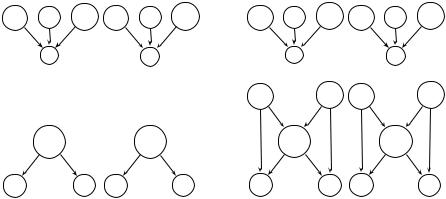
Fig. 9.3. The transformation in Step 2 of the decision procedure

Given a quantifier-free conjunctive Σcons-formula F , ¬atom(ui) literals are removed in a preprocessing step that follows from the (construction) axiom. Replace

¬atom(ui) with ui = cons(u1i , u2i ) .

Now consider Σcons-formula

F : s1 = t1 · · · sm = tm sm+1 6=tm+1 · · · sn 6=tn

atom(u1) · · · atom(uℓ)

in which si, ti, and ui are Tcons-terms. To decide its Tcons-satisfiability, perform the following steps:

1.Construct the initial DAG for the subterm set SF .

2.For each node n such that n.fn = cons,

•add car(n) to the DAG and merge car(n) n.args[1];

•add cdr(n) to the DAG and merge cdr(n) n.args[2]

by the (left projection) and (right projection) axioms. See Figure 9.3.

3.For i {1, . . . , m}, merge si ti.

4.For i {m + 1, . . . , n}, if find si = find ti, return unsatisfiable.

5.For i {1, . . . , ℓ} if v. find v = find ui v.fn = cons, return unsatisfiable by axiom (atom).

6.Otherwise, return satisfiable.

Steps 1, 3, 4, and 6 are identical to Steps 1-4 of the decision procedure for TE. Because of their similarity, it is simple to combine the two theories.

Example 9.20. Consider the (Σcons ΣE)-formula

F : car(x) = car(y) cdr(x) = cdr(y) f (x) 6=f (y)

¬atom(x) ¬atom(y)

in which the function symbol f is in Σ=. Is it (Tcons TE)-satisfiable? According to the final two literals, x and y are non-atom structures; thus, the first two literals imply that x = y. Yet the third literal, f (x) 6=f (y), contradicts this

Fig. 9.4. DAG after (a) Step 1 and (b) Step 2

equality according to the (congruence) axiom of TE. Hence, F is (Tcons TE)- unsatisfiable.

To prepare F for the decision procedure, rewrite F according to the (construction) axiom:

F ′ : car(x) = car(y) cdr(x) = cdr(y) f (x) 6=f (y)

x = cons(u1, v1) y = cons(u2, v2) .

The first two and final two literals imply that u1 = u2 and v1 = v2 so that again x = y. The remaining reasoning is as for F .

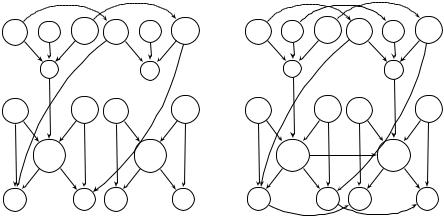
Let us apply the decision procedure to F ′. The initial DAG of F ′ is displayed in Figure 9.4(a). Figure 9.4(b) displays the DAG after Step 2.

According to the literals car(x) = car(y) and cdr(x) = cdr(y), compute

merge car(x) car(y) and merge cdr(x) cdr(y) ,

which add the two dashed arrows on the top of Figure 9.5(a). Then according to literal x = cons(u1, v1),

merge x cons(u1, v1) ,

which adds the dashed arrow from x to cons in Figure 9.5(a). Consequently, car(x) and car(cons(u1, v1)) become congruent. Since

find car(x) = car(y) and find car(cons(u1, v1)) = u1 ,

the find of car(y) is set to point to u1 during the subsequent union, resulting in the left dotted arrow of Figure 9.5(a). Similarly, cdr(x) and cdr(cons(u1, v1)) become congruent, with similar e ects (the right dotted arrow of Figure

262 9 Quantifier-Free Equality and Data Structures

Fig. 9.5. (a) Intermediate DAG and (b) final DAG

9.5(a)). The state of the DAG after these merges is shown in Figure 9.5(a). Dashed lines indicate merges that arise directly from the literals of F ′; dotted lines indicate deduced merges.

Next, according to the literal y = cons(u2, v2),

merge y cons(u2, v2) ,

resulting in the new dashed line from y to cons(u2, v2) in Figure 9.5(b). This merge produces two new congruences:

car(y) = car(cons(u2, v2)) and cdr(y) = cdr(cons(u2, v2)) .

Trace through the actions of these merges to understand the addition of the two bottom dotted arrows from u1 to u2 and from v1 to v2 in Figure 9.5(b). During the computation

merge cdr(y) cdr(cons(u2, v2)) ,

cons(u1, v1) and cons(u2, v2) become congruent; then find of cons(u1, v1) is set to point to cons(u2, v2), as represented by the new horizontal dashed line in Figure 9.5(b). This congruence causes the additional congruence

f (x) = f (y) ;

merge f (x) f (y) produces the final dotted edge from f (x) to f (y). Figure 9.5(b) displays the final DAG.

Does this DAG model F ? No, as find f (x) is f (y) and find f (y) is f (y) so

that f (x) f (y); however, F asserts that f (x) 6=f (y). F is thus (Tcons TE )- unsatisfiable.

9.5 Arrays

Arrays are a basic nonrecursive data type in programming languages, so reasoning about them is important. In this section, we present a decision procedure for the quantifier-free fragment of TA. This fragment is not expressive: one can assert properties only of individual elements, not of entire arrays. Chapter 11 examines a decision procedure for a more expressive fragment.

Recall from Chapter 3 that the theory of arrays TA has signature

ΣA : {·[·], ·h· ·i, =} ,

where

•a[i] is a binary function: a[i] represents the value of array a at position i;

•ahi vi is a ternary function: ahi vi represents the modified array a in which position i has value v;

•and = is a binary predicate.

The axioms of TA are the following:

1.the axioms of (reflexivity), (symmetry), and (transitivity) of TE

We consider TA-satisfiability in the quantifier-free fragment of TA. As usual, we consider only conjunctive ΣA-formulae since conversion to DNF extends the decision procedure to arbitrary quantifier-free ΣA-formulae.

The decision procedure for TA-satisfiability of quantifier-free ΣA-formula F is based on a reduction to TE-satisfiability via applications of the (read-over- write) axioms. Intuitively, if F does not contain any write terms, then the read terms can be viewed as uninterpreted function terms. Otherwise, any write term must occur in the context of a read — as a read-over-write term ahi vi[j]

— since arrays themselves cannot be asserted to be equal or not equal. In this case, the (read-over-write) axioms can be applied to deconstruct the read- over-write terms. In detail, to decide the TA-satisfiability of F , perform the following recursive steps.

Step 1

If F does not contain any write terms ahi vi, perform the following steps:

1.Associate each array variable a with a fresh function symbol fa, and replace each read term a[i] with fa(i).

2.Decide and return the TE-satisfiability of the resulting formula.

264 9 Quantifier-Free Equality and Data Structures

Step 2

Select some read-over-write term ahi vi[j] (recall that a may itself be a write term), and split on two cases:

1. According to (read-over-write 1), replace

F [ahi vi[j]] with F1 : F [v] i = j ,

and recurse on F1. If F1 is found to be TA-satisfiable, return satisfiable. 2. According to (read-over-write 2), replace

F [ahi vi[j]] with F2 : F [a[j]] i 6=j ,

and recurse on F2. If F2 is found to be TA-satisfiable, return satisfiable.

If both F1 and F2 are found to be TA-unsatisfiable, return unsatisfiable.

Example 9.21. Consider ΣA-formula

F : i1 = j i1 6=i2 a[j] = v1 ahi1 v1ihi2 v2i[j] 6=a[j] .

Recall that ahi1 v1ihi2 v2i[j] abbreviates the term

((ahi1 v1i)hi2 v2i)[j] .

F contains a write term, so select a read-over-write term to deconstruct:

ahi1 v1ihi2 v2i[j] .

According to (read-over-write 1), assume i2 = j and recurse on

F1 : i2 = j i1 = j i1 6=i2 a[j] = v1 v2 6=a[j] .

F1 does not contain any write terms, so rewrite it to

F1′ : i2 = j i1 = j i1 6=i2 fa(j) = v1 v2 6=fa(j) .

The first two literals imply that i1 = i2, contradicting the third literal, so F1′ is TE-unsatisfiable.

Returning, we try the second case: according to (read-over-write 2), assume i2 6=j and recurse on

F2 : i2 6=j i1 = j i1 6=i2 a[j] = v1 ahi1 v1i[j] 6=a[j] .

F2 contains a write term, so select the only read-over-write term to deconstruct. According to (read-over-write 1), assume i1 = j and recurse on

F3 : i1 = j i2 6=j i1 = j i1 6=i2 a[j] = v1 v1 6=a[j] .

Clearly, following this path leads to a contradiction because of the final two terms. Thus, according to (read-over-write 2), assume i1 6=j and recurse on

F4 : i1 6=j i2 6=j i1 = j i1 6=i2 a[j] = v1 a[j] 6=a[j] .

But the final literal is contradictory. As all branches have been tried, F is TA-unsatisfiable.

Theorem 9.22 (Sound & Complete). Given quantifier-free conjunctive ΣA-formula F , the decision procedure returns satisfiable i F is TA-satisfiable; otherwise, it returns unsatisfiable.

Theorem 9.23 (Complexity). TA-satisfiability of quantifier-free conjunctive ΣA-formulae is NP-complete.

The power of disjunction manifested in Steps 2(a) and 2(b) of the decision procedure results in this complexity.

Proof. That the problem is in NP is simple: for a given formula F , guess a formula like F , except that for every instance of a read-over-write term ahi vi[j], it includes as a conjunction either i = j or i 6=j. Only a linear number of literals are added. Then check TA-satisfiability of this formula, using the new literals to simplify read-over-write terms.

To prove NP-hardness, we reduce from satisfiability of PL formulae, which is NP-complete. Given a propositional formula F in CNF, assert

vP 6=v¬P

for each variable P in F ; vP and v¬P represent the values of P and ¬P , respectively. Introduce a fresh constant •. Then consider the nth clause of F , say

(¬P Q ¬R) .

In this case, assert

a[jn] 6=• ahiP v¬P ihiQ vQihiR v¬Ri[jn] = • .

jn must be equal to one of the introduced values at iP , iQ, or iR. Therefore, at cell jn the corresponding value (v¬P , vQ, or v¬R) must equal •. In this fashion, add an assertion for each clause of F . Conjoin all assertions to form quantifier-free conjunctive ΣA-formula G. G is equisatisfiable to F : vP = • i P is true; and v¬P i P is false. G is also of size polynomial in the size of F . Thus, deciding TA-satisfiability of G decides propositional satisfiability of F , so TA-satisfiability is NP-complete.

9.6 Summary

This chapter presents the congruence closure algorithm and applications to

deciding satisfiability in the quantifier-free fragments of TE, Tcons, and TA. It covers:

•The congruence closure algorithm at an abstract level. Relations, equivalence relations, congruence relations. Partitions; equivalence and congruence classes. Closures.

266 9 Quantifier-Free Equality and Data Structures

•The DAG-based implementation. Directed acyclic graph representation of formulae. The union-find algorithm. Merging.

•Recursive data structures. These structures include records, lists, stacks, and trees, but not queues. The decision procedure extends the congruence closure algorithm.

•Arrays. The decision procedure branches based on read-over-write terms according to the read-over-write axioms. When all write terms have been removed on one branch, the congruence closure algorithm is applied.

Equality is found within many first-order theories, including all the theories studied in this book. Additionally, equality and the congruence closure algorithm are the unifying components of the Nelson-Oppen combination method studied in Chapter 10. Hence, reasoning about it is fundamental. Fortunately, satisfiability is e ciently decidable using the congruence closure algorithm.

Uninterpreted functions are used to represent data structures in the context of TRDS and TA. In applications such as software and hardware verification, they allow abstracting away implementations of select components to simplify reasoning.

The DAG-based data structure that is the basis of the congruence closure algorithm is used whenever subformulae must be represented uniquely, either for algorithm correctness or for space and time considerations. Exercises 9.4 and 9.5 explore this data structure.

So far, we have seen three types of decision procedures. The quantifierelimination procedures of Chapter 7 manipulate formulae to construct equivalent quantifier-free (and possibly variable-free) formulae. The simplex method of Chapter 8 works explicitly with the underlying structure of the set of satisfying interpretations. The congruence closure algorithm shares characteristics of both types of procedures: it manipulates formulae e ciently using the DAGbased algorithm; but it also represents satisfying interpretations explicitly as congruence classes of terms via the find pointers.

Bibliographic Remarks

The quantifier-free fragment of TE was first proved decidable by Ackermann in 1954 [1] and later studied by various teams in the late 1970s. Shostak [83], Nelson and Oppen [66], and Downey, Sethi, and Tarjan [29] present alternate solutions to the problem. We discuss the method of Nelson and Oppen [66].

Oppen presents a theory of acyclic recursive data structures [69, 71]. The decision problem in the quantifier-free fragment of this theory is decidable in linear time, and the full theory is decidable. Our presentation is based on the work of Nelson and Oppen [66] for possibly-cyclic data structures.

McCarthy proposes the axiomatization of arrays based on read-over-write [58]. James King implemented the decision procedure for the quantifier-free fragment as part of his thesis work [50].

268 9 Quantifier-Free Equality and Data Structures

9.8 (DP for quantifier-free TA). Apply the decision procedure for quantifierfree TA to the following ΣA-formulae.

(a) ahi ei[j] = e i 6=j

(b) ahi ei[j] = e a[j] 6=e

(c) ahi ei[j] = e i 6=j a[j] 6=e

(d) ahi eihj f i[k] = g j 6=k i = j a[k] 6=g (e) i1 = j a[j] = v1 ahi1 v1ihi2 v2i[j] 6=a[j]