

Теория информации / Cover T.M., Thomas J.A. Elements of Information Theory. 2006., 748p
.pdf9.4 PARALLEL GAUSSIAN CHANNELS |
275 |
Z1
X1 |
Y1 |
Zk
Xk |
Yk |
FIGURE 9.3. Parallel Gaussian channels.
We calculate the distribution that achieves the information capacity for this channel. The fact that the information capacity is the supremum of achievable rates can be proved by methods identical to those in the proof of the capacity theorem for single Gaussian channels and will be omitted.
Since Z1, Z2, . . . , Zk are independent,
I (X1, X2, . . . , Xk ; Y1, Y2, . . . , Yk )
=h(Y1, Y2, . . . , Yk ) − h(Y1, Y2, . . . , Yk |X1, X2, . . . , Xk )
=h(Y1, Y2, . . . , Yk ) − h(Z1, Z2, . . . , Zk |X1, X2, . . . , Xk )
= h(Y1, Y2 |
, . . . , Yk ) − h(Z1, Z2, . . . , Zk ) |
(9.68) |
|||||
= h(Y1, Y2 |
, . . . , Yk ) − h(Zi ) |
(9.69) |
|||||
|
|
|
|
|
|
i |
|
≤ h(Yi ) − h(Zi ) |
|
(9.70) |
|||||
i |
|
|
|
|
|
|
|
≤ |
2 |
|
|
+ Ni |
|
|
|
|
1 |
log 1 |
|
Pi |
, |
(9.71) |
|
|
|
|
|
||||
i
9.5 CHANNELS WITH COLORED GAUSSIAN NOISE |
277 |
Power 
n
P1
P2
N3
N1
N2
Channel 1 |
Channel 2 |
Channel 3 |
FIGURE 9.4. Water-filling for parallel channels.
noise. When the available power is increased still further, some of the power is put into noisier channels. The process by which the power is distributed among the various bins is identical to the way in which water distributes itself in a vessel, hence this process is sometimes referred to as water-filling.
9.5CHANNELS WITH COLORED GAUSSIAN NOISE
In Section 9.4, we considered the case of a set of parallel independent Gaussian channels in which the noise samples from different channels were independent. Now we will consider the case when the noise is dependent. This represents not only the case of parallel channels, but also the case when the channel has Gaussian noise with memory. For channels with memory, we can consider a block of n consecutive uses of the channel as n channels in parallel with dependent noise. As in Section 9.4, we will calculate only the information capacity for this channel.
Let KZ be the covariance matrix of the noise, and let KX be the input covariance matrix. The power constraint on the input can then be written as
1 |
EXi2 ≤ P , |
(9.79) |
|||
|
n |
||||
|
|
|
i |
|
|
or equivalently, |
|
|
|
|
|
|
|
1 |
tr(KX) |
≤ P . |
(9.80) |
|
|
|
|||
|
|
n |
|||

278 GAUSSIAN CHANNEL
Unlike Section 9.4, the power constraint here depends on n; the capacity will have to be calculated for each n.
Just as in the case of independent channels, we can write
I (X1, X2, . . . , Xn; Y1, Y2, . . . , Yn) = h(Y1, Y2, . . . , Yn)
− h(Z1, Z2, . . . , Zn). (9.81)
Here h(Z1, Z2, . . . , Zn) is determined only by the distribution of the noise and is not dependent on the choice of input distribution. So finding the capacity amounts to maximizing h(Y1, Y2, . . . , Yn). The entropy of the output is maximized when Y is normal, which is achieved when the input is normal. Since the input and the noise are independent, the covariance of the output Y is KY = KX + KZ and the entropy is
|
1 |
(2π e)n|KX + KZ | . |
|
h(Y1, Y2, . . . , Yn) = |
2 log |
(9.82) |
Now the problem is reduced to choosing KX so as to maximize |KX + KZ |, subject to a trace constraint on KX. To do this, we decompose KZ into its diagonal form,
KZ = Q Qt , where QQt = I. |
(9.83) |
Then |
|
|KX + KZ | = |KX + Q Qt | |
(9.84) |
= |Q||Qt KXQ + ||Qt | |
(9.85) |
= |Qt KXQ + | |
(9.86) |
= |A + |, |
(9.87) |
where A = Qt KXQ. Since for any matrices B and C, |
|
tr(BC) = tr(CB), |
(9.88) |
we have |
|
tr(A) = tr(Qt KXQ) |
(9.89) |
= tr(QQt KX) |
(9.90) |
= tr(KX). |
(9.91) |
9.5 CHANNELS WITH COLORED GAUSSIAN NOISE |
279 |
Now the problem is reduced to maximizing |A + | subject to a trace constraint tr(A) ≤ nP .
Now we apply Hadamard’s inequality, mentioned in Chapter 8. Hadamard’s inequality states that the determinant of any positive definite matrix
K is less than the product of its diagonal elements, that is, |
|
|K| ≤ " Kii |
(9.92) |
i |
|
with equality iff the matrix is diagonal. Thus, |
|
|A + | ≤ "(Aii + λi ) |
(9.93) |
i |
|
with equality iff A is diagonal. Since A is subject to a trace constraint,
1 |
Aii ≤ P , |
(9.94) |
|
|
n |
||
|
|
i |
|
and Aii ≥ 0, the maximum value of #i (Aii + λi ) is attained when |
|||
|
Aii + λi = ν. |
(9.95) |
|
However, given the constraints, it may not always be possible to satisfy this equation with positive Aii . In such cases, we can show by the standard Kuhn–Tucker conditions that the optimum solution corresponds to setting
Aii = (ν − λi )+, |
(9.96) |
where the water level ν is chosen so that Aii = nP . This value of A maximizes the entropy of Y and hence the mutual information. We can use Figure 9.4 to see the connection between the methods described above and water-filling.
Consider a channel in which the additive Gaussian noise is a stochastic process with finite-dimensional covariance matrix KZ(n). If the process is stationary, the covariance matrix is Toeplitz and the density of eigenvalues on the real line tends to the power spectrum of the stochastic process [262]. In this case, the above water-filling argument translates to water-filling in the spectral domain.
Hence, for channels in which the noise forms a stationary stochastic process, the input signal should be chosen to be a Gaussian process with a spectrum that is large at frequencies where the noise spectrum is small.
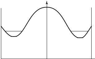
280 GAUSSIAN CHANNEL
F(w)
 w
w
FIGURE 9.5. Water-filling in the spectral domain.
This is illustrated in Figure 9.5. The capacity of an additive Gaussian noise channel with noise power spectrum N (f ) can be shown to be [233]
C |
= |
π |
1 |
log 1 |
+ |
(ν − N (f ))+ |
df, |
(9.97) |
|
|
|||||||
|
−π 2 |
N (f ) |
|
|||||
where ν is chosen so that $ (ν − N (f ))+ df = P .
9.6GAUSSIAN CHANNELS WITH FEEDBACK
In Chapter 7 we proved that feedback does not increase the capacity for discrete memoryless channels, although it can help greatly in reducing the complexity of encoding or decoding. The same is true of an additive noise channel with white noise. As in the discrete case, feedback does not increase capacity for memoryless Gaussian channels.
However, for channels with memory, where the noise is correlated from time instant to time instant, feedback does increase capacity. The capacity without feedback can be calculated using water-filling, but we do not have a simple explicit characterization of the capacity with feedback. In this section we describe an expression for the capacity in terms of the covariance matrix of the noise Z. We prove a converse for this expression for capacity. We then derive a simple bound on the increase in capacity due to feedback.
The Gaussian channel with feedback is illustrated in Figure 9.6. The output of the channel Yi is
Yi = Xi + Zi , Zi N(0, KZ(n)). |
(9.98) |
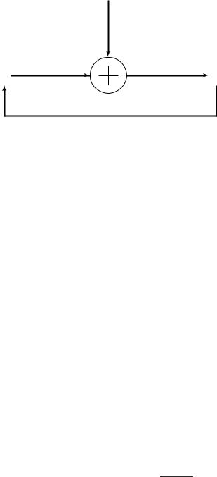
9.6 GAUSSIAN CHANNELS WITH FEEDBACK |
281 |
Zi
Xi |
Yi |
FIGURE 9.6. Gaussian channel with feedback.
The feedback allows the input of the channel to depend on the past values of the output.
A (2nR , n) code for the Gaussian channel with feedback consists of a sequence of mappings xi (W, Y i−1), where W {1, 2, . . . , 2nR } is the
input message and Y i−1 is the sequence of past values of the output. Thus, x(W, ·) is a code function rather than a codeword. In addition, we require that the code satisfy a power constraint,
1 |
n |
|
|
E% |
|
xi2(w, Y i−1)& ≤ P , w {1, 2, . . . , 2nR }, |
(9.99) |
n |
|||
|
|
i=1 |
|
where the expectation is over all possible noise sequences.
We characterize the capacity of the Gaussian channel is terms of the covariance matrices of the input X and the noise Z. Because of the feedback, Xn and Zn are not independent; Xi depends causally on the past values of Z. In the next section we prove a converse for the Gaussian channel with feedback and show that we achieve capacity if we take X to be Gaussian.
We now state an informal characterization of the capacity of the channel with and without feedback.
1.With feedback . The capacity Cn,FB in bits per transmission of the time-varying Gaussian channel with feedback is
C |
n,FB = |
max |
1 |
log |
|KX(n)+Z | |
, |
(9.100) |
|
|||||||
|
n1 tr(KX(n))≤P 2n |
|
|KZ(n)| |
|
|||
9.6 GAUSSIAN CHANNELS WITH FEEDBACK |
283 |
We now prove an upper bound for the capacity of the Gaussian channel with feedback. This bound is actually achievable [136], and is therefore the capacity, but we do not prove this here.
Theorem 9.6.1 For a Gaussian channel with feedback, the rate Rn for any sequence of (2nRn , n) codes with Pe(n) → 0 satisfies
Rn ≤ Cn,F B + n, |
(9.107) |
with n → 0 as n → ∞, where Cn,F B is defined in (9.100).
Proof: Let W be uniform over 2nR , and therefore the probability of error Pe(n) is bounded by Fano’s inequality,
ˆ |
(n) |
= n n, |
(9.108) |
H (W |W ) ≤ 1 |
+ nRnPe |
where n → 0 as Pe(n) → 0. We can then bound the rate as follows:
nRn = H (W ) |
|
|
|
(9.109) |
|
= |
ˆ |
ˆ |
|
|
(9.110) |
I (W ; W ) + H (W |W ) |
|
|
|||
|
ˆ |
|
|
|
(9.111) |
≤ I (W ; W ) + n n |
|
|
|
||
≤ I (W ; Y n) + n n |
|
|
|
(9.112) |
|
= I (W ; Yi |Y i−1) + n n |
|
|
(9.113) |
||
(a) |
h(Yi |Y i−1) − h(Yi |W, Y i−1 |
, Xi , Xi−1 |
, Zi−1) |
+ n n |
|
= |
|||||
|
|
|
|
|
(9.114) |
(b) |
h(Yi |Y i−1) − h(Zi |W, Y i−1, Xi , Xi−1, Zi−1) |
+ n n |
|||
= |
|||||
|
|
|
|
|
(9.115) |
(c) |
h(Yi |Y i−1) − h(Zi |Zi−1) + n n |
|
(9.116) |
||
= |
|
||||
= h(Y n) − h(Zn) + n n, |
|
|
(9.117) |
||
where (a) follows from the fact that Xi is a function of W and the past Yi ’s, and Zi−1 is Y i−1 − Xi−1, (b) follows from Yi = Xi + Zi and the
fact that h(X + Z|X) = h(Z|X), and (c) follows from the fact Zi and (W, Y i−1, Xi ) are conditionally independent given Zi−1. Continuing the
284 GAUSSIAN CHANNEL
chain of inequalities after dividing by n, we have |
|
||||||||
1 |
h(Y n) − h(Zn) + n |
(9.118) |
|||||||
Rn ≤ |
|
||||||||
n |
|||||||||
|
1 |
log |
|KY(n)| |
|
|
|
(9.119) |
||
≤ 2n |
|KZ(n)| + |
n |
|||||||
|
|
(9.120) |
|||||||
≤ Cn,F B + n, |
|
|
|||||||
by the entropy maximizing property of the normal. |
|
||||||||
We have proved an upper bound on the capacity of the Gaussian channel with feedback in terms of the covariance matrix KX(n)+Z . We now derive
bounds on the capacity with feedback in terms of KX(n) and KZ(n), which will then be used to derive bounds in terms of the capacity without feedback. For simplicity of notation, we will drop the superscript n in the symbols for covariance matrices.
We first prove a series of lemmas about matrices and determinants.
Lemma 9.6.1 Let X and Z be n-dimensional random vectors. Then
KX+Z + KX−Z = 2KX + 2KZ . |
(9.121) |
Proof |
|
KX+Z = E(X + Z)(X + Z)t |
(9.122) |
= EXXt + EXZt + EZXt + EZZt |
(9.123) |
= KX + KXZ + KZX + KZ . |
(9.124) |
Similarly, |
|
KX−Z = KX − KXZ − KZX + KZ . |
(9.125) |
Adding these two equations completes the proof. |
|
Lemma 9.6.2 For two n × n nonnegative definite matrices A and B, if A − B is nonnegative definite, then |A| ≥ |B|.
Proof: Let C = A − B. Since B and C are nonnegative definite, we can consider them as covariance matrices. Consider two independent normal random vectors X1 N(0, B) and X2 N(0, C). Let Y = X1 + X2.