Теория информации / Cover T.M., Thomas J.A. Elements of Information Theory. 2006., 748p

where the substitution g log φK = φK log φK follows from the fact

that g and φK yield the same moments of the quadratic form log φK (x).

In particular, the Gaussian distribution maximizes the entropy over all distributions with the same variance. This leads to the estimation counterpart to Fano’s inequality. Let X be a random variable with differ-

the expected prediction error. Let h(X) be in nats.

Theorem 8.6.6 (Estimation error and differential entropy ) For any

with equality if and only if is Gaussian and ˆ is the mean of .

X X X

where (8.78) follows from the fact that the mean of X is the best estimator for X and the last inequality follows from the fact that the Gaussian

PROBLEMS 257

(b)The Laplace density, f (x) = 12 λe−λ|x|.

(c)The sum of X1 and X2, where X1 and X2 are independent normal random variables with means µi and variances σi2, i = 1, 2.

8.2Concavity of determinants. Let K1 and K2 be two symmetric nonnegative definite n × n matrices. Prove the result of Ky Fan [199]:

| λK1 + λK2 |≥| K1 |λ| K2 |λ for 0 ≤ λ ≤ 1, λ = 1 − λ,

where | K | denotes the determinant of K. [Hint: Let Z = Xθ , where X1 N (0, K1), X2 N (0, K2) and θ = Bernoulli(λ). Then use h(Z | θ ) ≤ h(Z).]

8.3Uniformly distributed noise. Let the input random variable X to

a channel be uniformly distributed over the interval − 12 ≤ x ≤ + 12 . Let the output of the channel be Y = X + Z, where the noise random variable is uniformly distributed over the interval −a/2 ≤ z ≤

+a/2.

(a)Find I (X; Y ) as a function of a.

(b)For a = 1 find the capacity of the channel when the input X

is peak-limited; that is, the range of X is limited to − 12 ≤ x ≤ + 12 . What probability distribution on X maximizes the mutual information I (X; Y )?

(c)(Optional ) Find the capacity of the channel for all values of a, again assuming that the range of X is limited to − 12 ≤ x ≤ + 12 .

8.4Quantized random variables. Roughly how many bits are required on the average to describe to three-digit accuracy the decay time (in years) of a radium atom if the half-life of radium is 80 years? Note that half-life is the median of the distribution.

8.5 Scaling . Let h(X) = − f (x) log f (x) dx. Show h(AX) = log | det(A) | + h(X).

8.6Variational inequality . Verify for positive random variables X that

to extremize J (Q) = EQ ln X−D(Q||P )+λ( Q(x)−1).

258DIFFERENTIAL ENTROPY

8.7Differential entropy bound on discrete entropy . Let X be a dis-

(8.95) [Hint: Construct a random variable X such that Pr(X = i) = pi . Let U be a uniform (0,1] random variable and let Y = X + U , where X and U are independent. Use the maximum entropy bound on Y to obtain the bounds in the problem. This bound is due to Massey (unpublished) and Willems (unpublished).]

8.8Channel with uniformly distributed noise. Consider a additive

channel whose input alphabet X = {0,±1,±2} and whose output Y = X+Z, where Z is distributed uniformly over the interval [−1, 1]. Thus, the input of the channel is a discrete random variable, whereas the output is continuous. Calculate the capacity C = maxp(x) I (X; Y ) of this channel.

8.9Gaussian mutual information. Suppose that (X, Y, Z) are jointly Gaussian and that X → Y → Z forms a Markov chain. Let X and

Y have correlation coefficient ρ1 and let Y and Z have correlation coefficient ρ2. Find I (X; Z).

8.11Nonergodic Gaussian process. Consider a constant signal V in

the presence of iid observational noise {Zi }. Thus, Xi = V + Zi , where V N (0, S) and Zi are iid N (0, N ). Assume that V and {Zi } are independent.

(a)Is {Xi } stationary?

(e) Does {Xi } have an AEP? That is, does − n1 log f (Xn) −→ h?

HISTORICAL NOTES

Differential entropy and discrete entropy were introduced in Shannon’s original paper [472]. The general rigorous definition of relative entropy and mutual information for arbitrary random variables was developed by Kolmogorov [319] and Pinsker [425], who defined mutual information as supP,Q I ([X]P; [Y ]Q), where the supremum is over all finite partitions P and Q.

262 GAUSSIAN CHANNEL

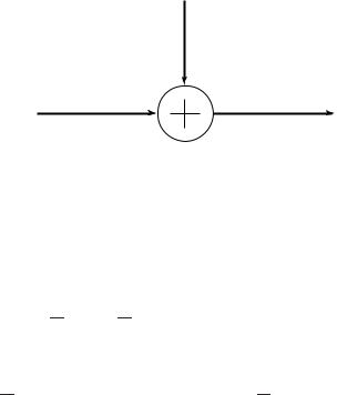
Zi

FIGURE 9.1. Gaussian channel.

cumulative effect of a large number of small random effects will be approximately normal, so the Gaussian assumption is valid in a large number of situations.

We first analyze a simple suboptimal way to use this channel. Assume that we want to send 1 bit over the channel in one use of the channel.

Given the power constraint, the best that we can do is to send one of

√ √

two levels, + P or − P . The receiver looks at the corresponding Y received and tries to decide which of the two levels was sent. Assuming that both levels are equally likely (this would be the case if we wish to

that + P was sent if Y > 0 and decide − P was sent if Y < 0. The probability of error with such a decoding scheme is

−∞

Using such a scheme, we have converted the Gaussian channel into a discrete binary symmetric channel with crossover probability Pe. Similarly, by using a four-level input signal, we can convert the Gaussian channel

into a discrete four-input channel. In some practical modulation schemes, similar ideas are used to convert the continuous channel into a discrete channel. The main advantage of a discrete channel is ease of processing of the output signal for error correction, but some information is lost in the quantization.

9.1GAUSSIAN CHANNEL: DEFINITIONS

We now define the (information) capacity of the channel as the maximum of the mutual information between the input and output over all distributions on the input that satisfy the power constraint.

Definition The information capacity of the Gaussian channel with power constraint P is

since X and Z are independent and EZ = 0. Given EY 2 = P + N , the entropy of Y is bounded by 12 log 2π e(P + N ) by Theorem 8.6.5 (the normal maximizes the entropy for a given variance).

Applying this result to bound the mutual information, we obtain

264 GAUSSIAN CHANNEL

EX ≤P

and the maximum is attained when X N(0, P ).

We will now show that this capacity is also the supremum of the rates achievable for the channel. The arguments are similar to the arguments for a discrete channel. We will begin with the corresponding definitions.

Definition An (M, n) code for the Gaussian channel with power constraint P consists of the following:

1.An index set {1, 2, . . . , M}.

2.An encoding function x : {1, 2, . . . , M} → Xn, yielding codewords xn(1), xn(2), . . . , xn(M), satisfying the power constraint P ; that is,

for every codeword

n

i=1

3. A decoding function

The rate and probability of error of the code are defined as in Chapter 7 for the discrete case. The arithmetic average of the probability of error is defined by

Definition A rate R is said to be achievable for a Gaussian channel with a power constraint P if there exists a sequence of (2nR , n) codes with codewords satisfying the power constraint such that the maximal probability of error λ(n) tends to zero. The capacity of the channel is the supremum of the achievable rates.

Theorem 9.1.1 The capacity of a Gaussian channel with power constraint P and noise variance N is