

Discrete.Math.in.Computer.Science,2002
.pdf5.2. UNIONS AND INTERSECTIONS |
163 |
23.In how many ways may we place n distinct books on k shelves so that shelf one gets at least m books? (See Exercise ??-8.) In how many ways may we place n distinct books on k shelves so that no shelf gets more than m books?
164 |
CHAPTER 5. PROBABILITY |
5.3Conditional Probability and Independence
Conditional Probability
Two cubical dice each have a triangle painted on one side, a circle painted on two sides and a square painted on three sides. Applying the principal of inclusion and exclusion, we can compute that the probability that we see a circle on at least one top when we roll them is 1/3 + 1/3 − 1/9 = 5/9. We are experimenting to see if reality agrees with our computation. We throw the dice onto the floor and they bounce a few times before landing in the next room.
5.3-1 Our friend in the next room tells us both top sides are the same. Now what is the probability that our friend sees a circle on at least one top?
Intuitively, it may seem as if the chance of getting circles ought to be four times the chance of getting triangles, and the chance of getting squares ought to be nine times as much as the chance of getting triangles. We could turn this into the algebraic statements that P (circles) = 4P (triangles) and P (squares) = 9P (triangles). These two equations and the fact that the probabilities sum to 1 would give us enough equations to conclude that the probability that our friend saw two circles is now 2/7. But does this analysis make sense? To convince ourselves, let us start with a sample space for the original experiment and see what natural assumptions about probability we can make to determine the new probabilities. In the process, we will be able to replace intuitive calculations with a formula we can use in similar situations. This is a good thing, because we have already seen situations where our intuitive idea of probability might not always agree with what the rules of probability give us.
Let us take as our sample space for this experiment the ordered pairs shown in Table 5.2 along with their probabilities.
|
|
|
Table 5.2: Rolling two unusual dice |
|
||||||||||||||
TT |
TC |
TS |
CT |
CC |
CS |
ST |
SC |
SS |
||||||||||
|
1 |
|
|
1 |
|
|
1 |
|
|
1 |
|
1 |
1 |
|
1 |
|
1 |
1 |
36 |
|
18 |
|
12 |
|
18 |
9 |
6 |
12 |
6 |
4 |
|||||||
We know that the event {TT, CC, SS} happened. Thus we would say while it used to have probability
1 |
+ |
1 |
+ |
1 |
= |
14 |
= |
7 |
(5.13) |
||
|
|
|
|
|
|
||||||
36 |
9 |
4 |
36 |
18 |
|||||||
|
|
|
|
|
|||||||
this event now has probability 1. Given that, what probability would we now assign to the event of seeing a circle? Notice that the event of seeing a circle now has become the event CC. Should we expect CC to become more or less likely in comparison than TT or SS just because we know now that one of these three outcomes has occurred? Nothing has happened to make us expect that, so whatever new probabilities we assign to these two events, they should have the same ratios as the old probabilities.
Multiplying all three old probabilities by 187 to get our new probabilities will preserve the ratios and make the three new probabilities add to 1. (Is there any other way to get the three new probabilities to add to one and make the new ratios the same as the old ones?) This gives

5.3. CONDITIONAL PROBABILITY AND INDEPENDENCE |
165 |
us that the probability of two circles is 19 · 187 = 27 . Notice that nothing we have learned about probability so far told us what to do; we just made a decision based on common sense. When faced with similar situations in the future, it would make sense to use our common sense in the same way. However, do we really need to go through the process of constructing a new sample space and reasoning about its probabilities again? Fortunately, our entire reasoning process can be captured in a formula. We wanted the probability of an event E given that the event F happened. We figured out what the event E ∩ F was, and then multiplied its probability by 1/P (F ). We summarize this process in a definition.
We define the conditional probability of E given F , denoted by P (E|F ) and read as “the
probability of E given F ” by |
|
P (E ∩ F ) |
|
|
P (E |
F ) = |
. |
(5.14) |
|
| |
|
P (F ) |
|
|
Then whenever we want the probability of E knowing that F has happened, we compute P (E|F ). (If P (F ) = 0, then we cannot divide by P (F ), but F gives us no new information about our situation. For example if the student in the next room says “A pentagon is on top,” we have no information except that the student isn’t looking at the dice we rolled! Thus we have no reason to change our sample space or the probability weights of its elements, so we define P (E|F ) = P (E) when P (F ) = 0.)
Notice that we did not prove that the probability of E given F is what we said it is; we simply defined it in this way. That is because in the process of making the derivation we made an additional assumption that the relative probabilities of the outcomes in the event F don’t change when F happens. We then made this assumption into part of our definition of what probability means by introducing the definition of conditional probability.4
In the example above, we can let E be the event that there is greater than one circle and F
be the event that both dice are the |
same. Then E |
∩ |
F is the event that both dice are circles, and |
|||||||
|
1 |
|
|
7 |
|
|||||
P (E |
∩ |
F ) is , from the table above, |
9 . |
P (F ) is, from Equation 5.13, |
|
. Dividing, we get the |
||||
18 |
||||||||||
|
1 |
7 |
2 |
|
|
|
||||
probability of P (E|F ), which is 9 / |
|
= |
7 . |
|
|
|
|
|||
18 |
|
|
|
|
||||||
5.3-2 When we roll two ordinary dice, what is the probability that the sum of the tops comes out even, given that the sum is greater than or equal to 10? Use the definition of conditional probability in solving the problem.
5.3-3 We say E is independent of F if P (E|F ) = P (E). Show that when we roll two dice, one red and one green, the event “The total number of dots on top is odd” is independent of the event “The red die has an odd number of dots on top.”
5.3-4 A test for a disease that a ects 0.1% of the population is 99% e ective on people with the disease (that is, it says they have it with probability 0.99). The test gives a false reading (saying that a person who does not have the disease is a ected with it) for 2% of the population without the disease. What is the probability that someone who has positive test results in fact has the disease?
For Exercise 5.3-2 let’s let E be the event that the sum is even and F be the event that the sum is greater than or equal to 10. Thus referring to our sample space in Exercise 5.3-2,
4For those who like to think in terms of axioms of probability, we simply added the axiom that the relative probabilities of the outcomes in the event F don’t change when F happens.

166 CHAPTER 5. PROBABILITY
P (F ) = 1/6 and P (E ∩ F ) = 1/9, since it is the probability that the roll is either 10 or 12. Dividing these two we get 2/3.
In Exercise 5.3-3, the event that the total number of dots is odd has probability 1/2. Similarly, given that the red die has an odd number of dots, the probability of an odd sum is 1/2 since this event corresponds exactly to getting an even roll on the green die. Thus, by the definition of independence, the event of an odd number of dots on the red die and the event that the total
number of dots is odd are independent. |
|
|
|
For Exercise 5.3-4, we are given that |
|
|
|
P (disease) = .001 , |
(5.15) |
||
P (positive test result|disease) = .99 , |
(5.16) |
||
P (positive test result|no disease) = .02 . |
(5.17) |
||
We wish to compute |
|
|
|
P (disease|positive test result) . |
|
||
We use Equation 5.14 to write that |
|
|
|
P (disease positive test result) = |
P (disease ∩ positive test result) |
. |
(5.18) |
| |
P (positive test result) |
|
|
How do we compute the numerator? |
Using the fact that P (disease ∩ positive test result) = |
|||
P (positive test result ∩ disease) and Equation 5.14 again, we can write |
||||
P (positive test result disease) = |
P (positive test result ∩ disease) |
. |
||
| |
|
P (disease) |
||
Plugging Equations 5.16 and 5.15 into this equation, we get |
||||
.99 = |
P (positive test result ∩ disease) |
|
||
|
|
.001 |
|
|
or P (positive test result ∩ disease) = (.001)(.99) = .00099. |
||||
To compute the denominator of Equation 5.18, we observe that since each person either has the disease or doesn’t, we can write
P (positive test result) = P (positive test result ∩ disease) + P (positive test result ∩ no disease) . (5.19)
We have already computed P (positive test result∩disease), and we can compute P (positive test result∩ no disease) in a similar manner. Writing
P (positive test result |
no disease) = |
P (positive test result ∩ no disease) |
, |
|
P (no disease) |
||||
| |
|
|
observing that P (no disease) = 1 − P (disease) and plugging in the values from Equations 5.15 and 5.17, we get that P (positive test result ∩no disease) = (.02)(1 −.001) = .01998 We now have the two components of the righthand side of Equation 5.19 and thus P (positive test result) =
.00099 + .01998 = .02097. Finally, we have all the pieces in Equation 5.18, and conclude that
P (disease |
positive test result) = |
P (disease ∩ positive test result) |
= |
.00099 |
= .0472 . |
|
P (positive test result) |
.02097 |
|||||
| |
|
|
|
Thus, given a test with this error rate, a positive result only gives you roughly a 5% chance of having the disease! This is another instance where probability shows something counterintuitive.

5.3. CONDITIONAL PROBABILITY AND INDEPENDENCE |
167 |
Independence
We said in Exercise 5.3-3 that E is independent of F if P (E|F ) = P (E). The product principle for independent probabilities (Theorem 5.3.1) gives another test for independence.
Theorem 5.3.1 Suppose E and F are events in a sample space. Then E is independent of F if and only if P (E ∩ F ) = P (E)P (F ).
Proof: First consider the case when F is non-empty. Then, from our definition in Exercise 5.3-3
E is independent of F P (E|F ) = P (E).
(Even though the definition only has an “if”, recall the convention of using “if” in definitions, even if “if and only if” is meant.) Using the definition of P (E|F ) in Equation 5.14, in the right side of the above equation we get
P (E|F ) = P (E)
P (E ∩ F ) = P (E) P (F )
P (E ∩ F ) = P (E)P (F ) .
Since every step in this proof was an if and only if statement we have completed the proof for the case when F is non-empty.
If F is empty, then E is independent of F and both P (E)P (F ) and P (E ∩ F ) are zero. Thus in this case as well, E is independent of F if and only if P (E ∩ F ) = P (E)P (F ). 
Corollary 5.3.2 E is independent of F if and only if F is independent of E.
When we flip a coin twice, we think of the second outcome as being independent of the first. It would be a sorry state of a airs if our definition did not capture this! For flipping a coin twice our sample space is {HH, HT, T H, T T } and we weight each of these outcomes 1/4. To say the second outcome is independent of the first, we must mean that getting an H second is independent of whether we get an H or a T first, and same for getting a T second. Note that
P (H first)P (H second) = 14 = P (H first and H second).
We can make a similar computation for each possible combination of outcomes for the first and second flip, and so we see that our definition of independence captures our intuitive idea of independence in this case. Clearly the same sort of computation applies to rolling dice as well.
5.3-5 What sample space and probabilities have we been using when discussing hashing? Using these, show that the event “key i hashes to position p” and the event “key j hashes to position q” are independent when i = j. Are they independent if i = j?
5.3-6 Show that if we flip a coin twice, the events E: “heads on the first flip,” F : “Heads on the second flip,” and H: “Heads on both flips” are each independent of the other two. Is
P (E ∩ F ∩ H) = P (E)P (F )P (H)?
Would it seem reasonable to say that these events are mutually independent?

168 |
CHAPTER 5. PROBABILITY |
Independent Trials Processes
Suppose we have a process that occurs in stages. (For example, we might flip a coin n times.) Let us use xi to denote the outcome at stage i. (For flipping a coin n times, xi = H means that the outcome of the ith flip is a head.) We let Si stand for the set of possible outcomes of stage i. (Thus if we flip a coin n times, Si = {H, T }.) A process that occurs in stages is called an independent trials process if for each sequence a1, a2, . . . , an with ai Si,
P (xi = ai|x1 = a1, . . . , xi−1 = ai−1) = P (xi = ai).
In other words, if we let Ei be the event that xi = ai, then
P (Ei|E1 ∩ E2 ∩ · · · ∩ Ei−1) = P (Ei).
By our product principle for independent probabilities, this implies that
P (E1 ∩ E2 ∩ · · · Ei−1 ∩ Ei) = P (E1 ∩ E2 ∩ · · · Ei−1)P (Ei). |
(5.20) |
Theorem 5.3.3 In an independent trials process the probability of a sequence a1, a2, . . . , an of outcomes is P ({a1})P ({a2}) · · · P ({an}).
Proof: We apply mathematical induction and Equation 5.20.
How does this reflect coin flipping? Here our sample space consists of sequences of Hs and T s, and the event that we have an H (or T ) on the ith flip is independent of the event that we have an H (or T ) on each of the first i −1 flips. Suppose we have a three-stage process consisting of flipping a coin, then flipping it again, and then computing the total number of heads. In this process, the outcome of the third stage is 2 if and only if the outcome of stage 1 is H and the outcome of stage 2 is H. Thus probability that the third outcome is 2, given that the first two are H is 1. Since the probability of two heads is 1/4 the third outcome is not independent of the first two. How do independent trials reflect hashing a list of keys? Here if we have a list of n keys to hash into a table of size k, our sample space consists of all n-tuples of numbers between 1 and k. The event that key i hashes to some number p is independent of the event that the first i − 1 keys hash to some number numbers q1, q2, qi−1. Thus our model of hashing is an independent trials process.
5.3-7 Suppose we draw a card from a standard deck of 52 cards, replace it, draw another card, and continue for a total of ten draws. Is this an independent trials process?
5.3-8 Suppose we draw a card from a standard deck of 52 cards, discard it (i.e. we do not replace it), draw another card and continue for a total of ten draws. Is this an independent trials process?
In Exercise 5.3-7 we have an independent trials process, because the probability that we draw a given card at one stage does not depend on what cards we have drawn in earlier stages. However, in Exercise 5.3-8, we don’t have an independent trials process. In the first draw, we have 52 cards to draw from, while in the second draw we have 51. Therefore we are not drawing from the same sample space. Further, the probability of getting a particular card on the ith draw increases as we draw more and more cards, unless we have already drawn this card, in which case the probability of getting this card drops to zero.
5.3. CONDITIONAL PROBABILITY AND INDEPENDENCE |
169 |
Binomial Probabilities
When we study an independent trials process with two outcomes at each stage, it is traditional to refer to those outcomes as successes and failures. When we are flipping a coin, we are often interested in the number of heads. When we are analyzing student performance on a test, we are interested in the number of correct answers. When we are analyzing the outcomes in drug trials, we are interested in the number of trials where the drug was successful in treating the disease. This suggests it would be interesting to analyze in general the probability of exactly k successes in n independent trials with probability p of success (and thus probability 1 − p of failure) on each trial. It is standard to call such an independent trials process a Bernoulli trials process.
5.3-9 Suppose we have 5 Bernoulli trials with probability p of success on each trial. What is the probability of success on the first three trials and failure on the last two? Failure on the first two trials and success on the last three? Success on trials 1, 3, and 5, and failure on the other two? Success on any three trials, and failure on the other two?
Since the probability of a sequence of outcomes is the product of the probabilities of the individual outcomes, the probability of any sequence of 3 successes and 2 failures is p3(1 − p)2. More generally, in n Bernoulli trials, the probability of a given sequence of k successes and n − k failures is pk (1 − p)n−k . However this is not the probability of having k successes, because many di erent sequences could have k successes.
How many sequences of n successes and failures have exactly k successes? The number of ways to choose the k places out of n where the successes occur is nk , so the number of sequences with k successes is nk . This paragraph and the last together give us Theorem 5.3.4.
Theorem 5.3.4 The probability of having exactly k successes in a sequence of independent trials with two outcomes and probability p of success on each trial is
P (exactly k successes) = |
n |
pk (1 − p)n−k |
k |
.
Proof: The proof follows from the two paragraphs preceding the theorem.
Because of the connection between these probabilities and the binomial coe cients, the probabilities of Theorem 5.3.4 are called binomial probabilities, or the binomial probability distribution.
5.3-10 A student takes a ten question objective test. Suppose that a student who knows 80% of the course material has probability .8 of success an any question, independently of how the student did on any other problem. What is the probability that this student earns a grade of 80 or better?
5.3-11 Recall the primality testing algorithm from Chapter ??. Here we said that we could, by choosing a random number less than or equal to n, perform a test on n that, if n was not prime, would certify this fact with probability 1/2. Suppose we perform 20 of these tests. It is reasonable to assume that each of these tests is independent of the rest of them. What is the probability that a non-prime number is certified to be non-prime?
170 |
CHAPTER 5. PROBABILITY |
Since a grade of 80 or better corresponds to 8, 9, or 10 successes in ten trials, in Exercise 5.3-10 we have
P (80 or better) = |
10 |
(.8)8(.2)2 + |
10 |
(.8)9(.2)1 + (.8)10. |
|
8 |
|
9 |
|
Some work with a calculator gives us that this sum is approximately .678.
In Exercise 5.3-11, we will first compute the probability that a non-prime number is not certified to be non-prime. If we think of success as when the number is certified non-prime and failure when it isn’t, then we see that the only way to fail to certify a number is to have 20 failures. Using our formula we see that the probability that a non-prime number is not certified non-prime is just 2020 (.5)20 = 1/1048576. Thus the chance of this happening is less than 1 in a million, and the chance of certifying the non-prime as non-prime is 1 minus this. Therefore it is almost sure that a non-prime number will be certified non-prime.
A Taste of Generating Functions We note a nice connection between the probability of having exactly k successes and the binomial theorem. Consider, as an example, the polynomial (H + T )3. Using the binomial theorem, we get that this is
(H + T )3 = |
3 |
H3 + |
3 |
H2T + |
3 |
HT 2 + |
3 |
T 3. |
|
0 |
|
1 |
|
2 |
|
3 |
|
We can interpret this as telling us that if we flip a coin three times, with outcomes heads or tails
each time, then there are |
3 |
= 1 way of getting 3 heads, |
3 |
= 3 ways of getting two heads and |
|||
|
3 |
|
0 |
|
2 |
3 |
|
one tail, |
= 3 ways of getting one head and two tails and |
= 1 way of getting 3 tails. |
|||||
|
1 |
|
|
|
|
3 |
|
Similarly, if instead of using H and T we put the probabilities of x times the probability of success and y times the probability of failure three independent trials in place of H and T we would get the following:
(px + (1 − p)y)3 = |
3 |
p3x3 + |
3 |
p2(1 − p)x2y + |
3 |
p(1 − p)2xy2 + |
3 |
(1 − p)3y3. |
0 |
1 |
2 |
3 |
Generalizing this to n repeated trials where in each trial the probability of success is p, we see that by taking (px + (1 − p)y)n we get
k
(px + (1 − p)y)n =
k=0
n pk (1 − p)n−k xk yn−k . k
Taking the coe cient of xk yn−k from this sum, we get exactly the result of Theorem 5.3.4. This connection is a simple case of a very powerful tool known as generating functions. We say that the polynomial (px + (1 − p)y)n generates the binomial probabilities.
Tree diagrams
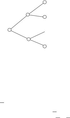
When we have a sample space that consists of sequences of outcomes, it is often helpful to visualize the outcomes by a tree digram. We will explain what we mean by giving a tree diagram

5.3. CONDITIONAL PROBABILITY AND INDEPENDENCE |
171 |
Figure 5.1: A tree diagram illustrating a two-stage process.
|
|
D |
|
|
.5 |
.1 |
|
N |
|
||
.5 |
Q |
||
|
|||
|
|
.1 |
.2 N
|
.25 |
.1 |
|
D |
|
D |
|
.4 |
.25 |
||
|
|
.1 |
|
|
.5 |
Q |
|
|
.2 |
||
|
|
||
.4 |
|
N |
|
|
.25 |
||
Q |
.1 |
||
.5 |
D |
||
|
|||
|
|
.2 |
|
|
.25 |
Q |
|
|
|
.1 |
of the following experiment. We have one nickel, two dimes, and two quarters in a cup. We draw a first and second coin. In Figure 5.3 you see our diagram for this process.
Each level of the tree corresponds to one stage of the process of generating a sequence in our sample space. Each vertex is labeled by one of the possible outcomes at the stage it represents. Each edge is labeled with a conditional probability, the probability of getting the outcome at its right end given the sequence of outcomes that have occurred so far. Since no outcomes have occurred at stage 0, we label the edges from the root to the first stage vertices with the probabilities of the outcomes at the first stage. Each path from the root to the far right of the tree represents a possible sequence of outcomes of our process. We label each leaf node with the probability of the sequence that corresponds to the path from the root to that node. By the definition of conditional probabilities, the probability of a path is the product of the probabilities along its edges. We draw a probability tree for any (finite) sequence of successive trials in this way.
Sometimes a probability tree provides a very e ective way of answering questions about a process. For example, what is the probability of having a nickel in our coin experiment? We see there are four paths containing an N , and the sum of their weights is .4, so the probability that one of our two coins is a nickel is .4.
5.3-12 How can we recognize from a probability tree whether it is the probability tree of an independent trials process?
5.3-13 Draw a tree diagram for Exercise 5.3-4 in which stage 1 is whether or not the person has the disease and stage two is the outcome of the test for the disease. Which branches of the tree correspond to the event of having a positive test? Describe the computation we made in Exercise 5.3-4 in terms of probabilities of paths from the root to leaves of the tree.
172 |
CHAPTER 5. PROBABILITY |
5.3-14 If a student knows 80% of the material in a a course, what do you expect her grade to be on a (well-balanced) 100 question short-answer test about the course? What do you expect her grade to be on a 100 question True-False test to be if she guesses at each question she does not know the answer to? (We assume that she knows what she knows, that is, if she thinks that she knows the answer, then she really does.)
A tree for an independent trials process has the property that at each non-leaf node, the (labeled) tree consisting of that node and all its children is identical to the labeled tree consisting of the root and all its children. If we have such a tree, then it automatically satisfies the definition of an independent trials process.
In Figure 5.3 we show the tree diagram for Exercise 5.3-4. We use D to stand for having
Figure 5.2: A tree diagram illustrating Exercise 5.3-4.
|
|
|
pos |
|
|
|
.0198 |
|
|
.02 |
|
|
ND |
|
neg |
|
|
|
|
.999 |
|
.98 |
.97902 |
|
|
pos
.99  .00099
.001
neg
D .01
.00001
the disease and ND to stand for not having the disease. The computation we made consisted of dividing the probability of the path root-D-pos by the sum of the probabilities of the paths root-ND-pos and root-D-pos.
In Exercise 5.3-14, if a student knows 80% of the material in a course, we would hope that her grade on a well-designed test of the course would be around 80%. But what if the test is a True-False test? Then as we see in Figure 5.3 she actually has probability .9 of getting a right answer if she guesses at each question she does not know the answer to. We can also write this out algebraically. Let R be the event that she gets the right answer, K be the event that she knows that right answer and K be the event that she guesses. Then,
P (R) = P (R ∩ K) + P (R ∩ K)
=P (R|K)P (K) + P (R|K)P (K)
=1 · .8 + .5 · .2 = .9
Thus we would expect her to get a grade of 90%.
Problems
1.In three flips of a coin, what is the probability that two flips in a row are heads, given that there is an even number of heads?