Discrete.Math.in.Computer.Science,2002

The main idea is that the subsets of an n-element set can be partitioned by whether they contain element n or not. The subsets of {1, 2, . . . , n} containing element n can be constructed by adjoining the element n to the subsets without element n. So the number of subsets with element n is the same as the number of subsets without element n. The number of subsets without element n is just the number of subsets of an n − 1-element set. Thus the number of subsets of {1, 2, . . . , n} is twice the number of subsets of {1, 2, . . . , n − 1}. This will give us the inductive step of a proof by induction that the recurrence correctly describes the number of subsets of an n-element set for all n

How, exactly, does the inductive proof go? We know the initial condition of our recurrence properly describes the number of subsets of a zero-element set, namely 1 (remember that the empty set has itself and only itself as a subset). Now we suppose our recurrence properly describes the number of subsets of a k-element set for k less than n. Then since the number of subsets of an n-element set containing a specific element x is the same as the number of subsets without element x, the total number of number of subsets of an n-element set is just twice the number of subsets of an (n − 1)-element set. Therefore, because the recurrence properly describes the number of subsets of an (n − 1)-element subset, it properly describes the number of subsets of an n-element set. Therefore by the principle of mathematical induction, our recurrence describes the number of subsets of an n-element set for all integers n ≥ 0. Notice how the proof by induction goes along exactly the same lines as our derivation of the recurrence. This is one of the beautiful facets of the relationship between recurrences and induction; usually what we do to figure out a recurrence is exactly what we would do to prove we are right!

For Exercise 4.2-4 we can algebraically describe what the problem said in words by

T (n) = (1 + .01p/12) · T (n − 1) − M,

with T (0) = A. Note that we add .01p/12 times the principal to the amount due each month, because p/12 percent of a number is .01p/12 times the number.

Iterating a recurrence

Turning to Exercise 4.2-5, we can substitute the right hand side of the equation T (n − 1) = rT (n − 2) + a for T (n − 1) in our recurrence, and then substitute the similar equations for T (n − 2) and T (n − 3) to write

T (n) = r(rT (n − 2) + a) + a

=r2T (n − 2) + ra + a

=r2(rT (n − 3) + a) + ra + a

=r3T (n − 3) + r2a + ra + a

=r3(rT (n − 4) + a) + r2a + ra + a

=r4T (n − 4) + r3a + r2a + ra + a

From this, we can guess that

= rnb + ar − arn + a

1 − r

= rnb + ar − arn + a − ar

1 − r

= rnb + a 1 − rn .

1 − r

Therefore by the principle of mathematical induction, our formula holds for all integers n greater than 0.

Corollary 4.2.2 The formula for the sum of a geometric series with r = 1 is

n−1 ri = 1 − rn .

i=0

1 − r

Proof: Take b = 0 and a = 1 in Theorem 4.2.1. Then the sum 1 + r + · · · + rn−1 satisfies the recurrence given.

Often, when we see a geometric series, we will only be concerned with expressing the sum in big-O notation. In this case, we can show that the sum of a geometric series is at most the largest term times a constant factor, where the constant factor depends on r, but not on n.

Lemma 4.2.3 Let r be a quantity whose value is independent of n and not equal to 1. Let t(n) be the largest term of the geometric series

n−1

ri.

i=0

Then the value of the geometric series is O(t(n)).

Proof: It is straightforward to see that we may limit ourselves to proving the lemma for r > 0. We consider two cases, depending on whether r > 1 or r < 1. If r > 1, then

Theorem 4.2.5 For any positive constants a and r, and any function g defined on the nonnegative integers, the solution to the first order linear recurrence

i=1

Proof: Let’s prove this by induction.

Since the sum in equation 4.11 has no terms when n = 0, the formula gives T (0) = 0 and so is

valid when n = 0. We now assume that n is positive and T (n − 1) = rn−1a + n−1 r(n−1)−ig(i).

i=1

Using the definition of the recurrence and the inductive hypothesis we get that

T (n) = rT (n − 1) + g(n)

n−1

= r rn−1a + r(n−1)−ig(i) + g(n)

= rna + rn−ig(i).

i=1

Therefore by the principle of mathematical induction, the solution to

is given by Equation 4.11 for all nonnegative integers n.

The formula in Theorem 4.2.5 is a little less easy to use than that in Theorem 4.2.1, but for

a number of commonly occurring functions g the sum n rn−ig(i) is reasonable to compute.

i=1

4.2-6 Solve the recurrence T (n) = 4T (n − 1) + 2n with T (0) = 6.

Using Equation 4.11, we can write

=6 · 4n + (1 − ( 12 )n) · 4n

=7 · 4n − 2n

Problems

1.Solve the recurrence M (n) = 2M (n − 1) + 2, with a base case of M (1) = 1. How does it di er from the solution to Equation 4.7?

2.Solve the recurrence M (n) = 3M (n − 1) + 1, with a base case of M (1) = 1. How does it di er from the solution to Equation 4.7.

3.Solve the recurrence M (n) = M (n − 1) + 2, with a base case of M (1) = 1. How does it di er from the solution to Equation 4.7. Using iteration of the recurrence, we can write

M (n) = M (n − 1) + 2

=M (n − 2) + 2 + 2

=M (n − 3) + 2 + 2 + 2

.

.

.

=M (n − i) + 2 + 2 + · · · + 2 i times

=M (n − i) + 2i

Since we are given that M (1) is 1, we take i = n − 1 to get

=M (1) + 2(n − 1)

=1 + 2(n − 1)

=2n − 1

Now, we verify the correctness of our derivation through mathematical induction.

(a)Base Case : n = 1: M (1) = 2 · 1 − 1 = 1. Thus, base case is true.

(b)Suppose inductively that M (n − 1) = 2(n − 1) − 1. Now, for M (n), we have

M (n) = M (n − 1) + 2

= 2n − 2 − 1 + 2 = 2n − 1

So, from 1, 2 and the principle of mathematical induction, the statment is true for all n. We could have gotten the same result by using Theorem 4.2.1.

Here, the recurrence is of the form M (n) = M (n − 1) + 2 while in (4.8), it is of the form M (n) = 2M (n − 1) + 1. Thus, in Theorem 4.2.1, r would have been 1, and thus our geometric series sums to a multiple of the number of terms.

4.There are m functions from a one-element set to the set {1, 2, . . . , m}. How many functions are there from a two-element set to {1, 2, . . . , m}? From a three-element set? Give a recurrence for the number T (n) of functions from an n-element set to {1, 2, . . . , m}. Solve the recurrence.

5.Solve the recurrence that you derived in Exercise 4.2-4.

6.At the end of each year, a state fish hatchery puts 2000 fish into a lake. The number of fish in the lake at the beginning of the year doubles due to reproduction by the end of the year. Give a recurrence for the number of fish in the lake after n years and solve the recurrence.

7.Consider the recurrence T (n) = 3T (n − 1) + 1 with the initial condition that T (0) = 2. We know from Theorem 4.2.1 exactly what the solution is. Instead of using the theorem, try to guess the solution from the first four values of T (n) and then try to guess the solution by iterating the recurrence four times.

8.What sort of big-O bound can we give on the value of a geometric series 1 + r + r2 + · · ·+ rn with common ratio r = 1?

9.Solve the recurrence T (n) = 2T (n − 1) + n2n with the initial condition that T (0) = 1.

10.Solve the recurrence T (n) = 2T (n − 1) + n32n with the initial condition that T (0) = 2.

11.Solve the recurrence T (n) = 2T (n − 1) + 3n with T (0) = 1.

12.Solve the recurrence T (n) = rT (n − 1) + rn with T (0) = 1.

13.Solve the recurrence T (n) = rT (n − 1) + r2n with T (0) = 1

14.Solve the recurrence T (n) = rT (n − 1) + sn with T (0) = 1.

15.Solve the recurrence T (n) = rT (n − 1) + n with T (0) = 1. (There is a sum here that you

may not know; thinking about the derivative of 1 + x + x2 + · · · + xn will help you figure it out.)

a solution to the equation F (n) = F (n − 1) + F (n − 2) for any real numbers c1 and c2?

(d)Find constants c1 and c2 such that the Fibonacci numbers are given by

√√

4.3Rooted Trees

The idea of a rooted tree

You have seen trees as data structures for solving a variety of di erent kinds of problems. Mathematically speaking, a tree is a geometric figure consisting of vertices and edges—but of special kind. We think of vertices as points in the plane and we think of edges as line segments. In this section we will study some of the properties of trees that are useful in computer science. Most, but not all, of the trees we use in computer science have a special vertex called a root. Such trees are usually called “rooted trees.” We could certainly describe what we mean by a rooted tree in ordinary English. However it is particularly easy to give a recursive description of what we mean by a rooted tree. We say

A vertex P is a rooted tree with root P .

If T1, T2,...Tk are rooted trees with roots Ri, and P is a vertex, then drawing edges from P to each of the roots Ri gives a rooted tree T with root P . We call the trees T1, T2,...Tk subtrees of the root P our rooted tree T .

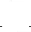
Any geometric figure we can construct by using these two rules is called a rooted tree. Just as we don’t really define points and lines in geometry, we won’t formally define the terms vertex and edge here. We do note that a standard synonym for vertex is node, and that edges represent relationships between vertices. In Figure 4.1 we show first a single vertex. We then imagine three trees which are copies of this single vertex and connect them to a new root. Finally we take two copies of the resulting tree and attach them to a new root.

Figure 4.1: The evolution of a rooted tree.

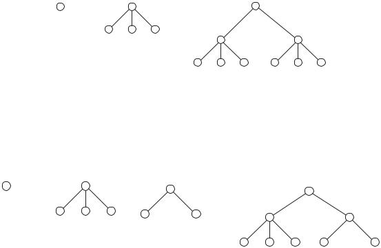
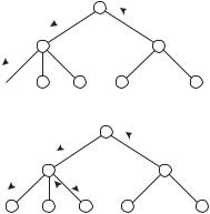
Of course we need not take multiple copies of the same tree. In Figure 4.2 we began as in Figure 4.1 but at the second stage, we created two di erent trees, one with two one-vertex trees attached to the root and one with three one-vertex trees attached to the root. Then at the third stage we attached the two trees from the second stage to a common root.

Figure 4.2: The evolution of a less symmetric rooted tree.

The number of vertices and edges in a tree

4.3-1 Draw 5 rooted trees with 7 vertices each. How many edges do they have? What do you think the relationship between the number of vertices and edges is in general. Prove that you are right.

In Exercise 4.3-1 you saw that each of your 7-vertex trees had six edges. This suggests a pattern, namely that a rooted tree with n vertices has n − 1 edges. How would we go about proving that? Well, a rooted tree with one vertex has no edges, because in our recursive definition the only way to get a tree with one vertex is to take a single vertex called a root. (That sounds like a base step for an inductive proof, doesn’t it?) If we have a rooted tree, it has a root vertex attached by edges to a certain number, say k, of trees. If these k trees have sizes n1, n2,. . . , nk , then we may assume inductively that they have n1 − 1, n2 − 1,. . . , nk − 1 edges respectively. (That should sound like the inductive hypothesis of an inductive proof.) If our original tree has

n vertices, then these trees have a total of n − 1 = k ni vertices and

i=1

(ni − 1) = ( ni) − k = n − 1 − k

edges. In addition to these vertices and edges, our original tree has 1 more vertex and k more edges (those that connect the subtrees to the root). Thus our original rooted tree has (n − 1 − k) + k = n − 1 edges. Therefore by the (strong) principle of mathematical induction, a rooted tree on n vertices has n − 1 edges.

Notice how this inductive proof mirrored the recursive definition of a rooted tree. Notice also that while it is an induction on the number n of vertices of the tree, we didn’t really mention n in our inductive hypothesis. So long as we have the correct structure for an inductive proof, it is quite acceptable to leave the number on which we are inducting implicit instead of explicit in our proof.

We have just proved the following theorem.

Theorem 4.3.1 A rooted tree with n vertices has n − 1 edges.

Paths in trees

A walk from vertex x to vertex y is an alternating sequence of vertices and edges starting at x and ending at y such that each edge connects the vertex that precedes it with the vertex that follows it. A path is a walk without repeated vertices. In Figure 4.3 we show a path from y to x by putting arrows beside its edges; we also show a walk that is not a path, using arrows with numbers to indicate its edges. In this walk, the vertex marked z is used twice (as is an edge).

4.3-2 Draw a rooted tree on 12 vertices. (Don’t draw a “boring” one.) Choose two vertices. Can you find a path between them. Can you find more than one? Try another two vertices. What do you think is true in general? Can you prove it?

How do we prove that there is exactly one path between any two vertices of a rooted tree? It is probably no surprise that we use induction. In particular, in a rooted tree with one vertex the

Figure 4.3: A path and a walk in a rooted tree.

y

x

z

y

5 3

4

x

only path or walk is the “alternating sequence of vertices and edges” that has no edges, namely that single vertex. That single vertex is the unique path from the vertex to itself, so in a tree with one vertex we have a unique path between any pair of vertices. Now let T be a rooted tree with root vertex r, and let T1, T2, . . . , Tk be the subtrees whose roots r1, r2, . . . , rk are joined to r by edges. Assume inductively that in each Ti there is a unique path between any pair of vertices. Then if we have a pair x and y of vertices in T , they are either in the same Ti (case 1), di erent subtrees Ti and Tj of the root (case 2), or one is the root and one is in a subtree Ti (case 3). In case 1, a walk from x to y that leaves tree Ti must enter it again, and so it must use vertex r twice. Thus the unique path between x and y in Ti is the unique path between x and y in T . In case 2 there is a unique path between x and ri in their subtree Ti and a unique path between rj and y in their subtree Tj . Thus in T we have a path from x to ri which we may follow with the edge from ri to r, then the vertex r, then the edge from r to rj , and finally the path from rj to y, which gives us a path from x to y.

Now we show that this is the unique path between x and y. When a path from x to y leaves Ti it must use the only edge that has one vertex in Ti and one vertex outside Ti, namely the edge from ri to r. To get to this edge, the path must follow the unique path from x to ri in Ti. The path continues along this edge to r. To get from r to y, the path must enter the subtree Tj , because y is in that subtree. When the path enters tree Tj , it must do so along the only edge that has one vertex in Tj and one vertex outside Tj , namely the edge from r to rj . Before it enters Tj , the path cannot go to any other root rk with k = j, thus entering tree Tk , because to get to y it would eventually have to leave the tree Tk and return to r in order to enter the tree Tj . But a walk that uses r twice would not be a path. Therefore the vertex following r in the path must be rj , and there is only one way to complete the path by going from rj to y in Tj . Therefore the path from x to y in T is unique.

Finally in case 3 suppose x is in the subtree Ti and y is the root of T . By our inductive hypothesis there is a unique in Ti from x to the root ri of Ti. Following this path with the edge from ri to r and the vertex r gives us a path from x to y since y = r. As before when a path leaves Ti it must go from ri to r along the unique edge connecting them. Since r is the last vertex twice, the path could not have any more edges or vertices or r would have to appear in the path a second time. However since there is only one path from x to ri, there is only one way for the path to reach ri. This means that the the path we described is the only possible one.