Discrete.Math.in.Computer.Science,2002

As we draw levels one and two, we see that at the level one, we have (3/4 + 1/5)n work. At the level two we have ((3/4)2 + 2(3/4)(1/5) + (1/5)2)n work. Were we to work out the third level we would see that we have ((3/4)3 + 3(3/4)2(1/5) + 3(3/4)(1/5)2 + (1/5)3)n. Thus we can see a pattern emerging. At level one we have (3/4 + 1/5)n work. At level 2 we have, by the binomial theorem, (3/4 + 1/5)2n work. At level 3 we have, by the binomial theorem, (3/4 + 1/5)3n work.

We have actually ignored one detail here. In contrast to a recursion tree in which all subproblems at a level has equal size, the “bottom” of the tree is more complicated. Di erent branches of the tree will reach 1 and terminate at di erent levels. For example, the branch that follows all 3/4’s will bottom out after log4/3 n levels, while the one that follows all 1/5’s will bottom out after log5 n levels. However, the analysis above overestimates the work, that is, it assumes that nothing bottoms out until log20/19 n levels, and in fact, the upper bound on the sum “assumes” that the recurrence never bottoms out.

We see here something general happening. It seems as if to understand a recurrence of the form T (n) = T (an)+T (bn)+O(n), we can study the simpler recurrence T (n) = T ((a+b)n)+O(n) instead. This simplifies things and allows us to analyze a larger class of recurrences. Turning to the median algorithm, it tells us that the important thing that happened there was that the size of the two recursive calls 3/4n and n/5 summed to less than 1. As long as that is the case for an algorithm, the algorithm will work in O(n) time.

Problems

1.In the MagicMiddle algorithm, suppose we broke our data up into n/3 sets of size 3. What would the running time of Select1 be?

2.In the MagicMiddle algorithm, suppose we broke our data up into n/7 sets of size 7. What would the running time of Select1 be?

Draw recursion trees for T and S. What are the big-O bounds we get on solutions to the recurrences? Use the recursion trees to argue that, for all n, T (n) ≤ S(n).

4.Find a (big-O) upper bound (the best you know how to get) on solutions to the recurrence T (n) = T (n/3) + T (n/6) + T (n/4) + n.

5.Find a (big-O) upper bound (the best you know how to get) on solutions the recurrence T (n) = T (n/4) + T (n/2) + n2.

6.Note that we have chosen the median of an n-element set to be the element in positionn/2 . We have also chosen to put the median of the medians into the set L of algorithm Select1. Show that this lets us prove that T (n) ≤ T (3n/4) + T (n/5) + cn for n ≥ 40 rather than n ≥ 60. (You will need to analyze the case where n/5 is even and the case where it is odd separately.)

believe to be the relative likelihood of that outcome. There are two rules we must follow in assigning weights. First the weights must be nonnegative numbers, and second the sum of the weights of all the elements in a sample space must be one. We define the probability P (E) of the event E to be the sum of the weights of the elements of E.

Notice that a probability function P on a sample space S satisfies the rules1

1.P (A) ≥ 0 for any A S.

2.P (S) = 1.

3.P (A B) = P (A) + P (B) for any two disjoint events A and B.

The first two rules reflect our rules for assigning weights above. We say that two events are disjoint if A ∩ B = . The third rule follows directly from the definition of disjoint and our definition of the probability of an event. A function P satisfying these rules is called a probability distribution or a probability measure.

In the case of the professor’s three question quiz, it is natural to expect each sequence of trues and falses to be equally likely. (A professor who showed any pattern of preferences would end up rewarding a student who observed this pattern and used it in educated guessing.) Thus it is natural to assign equal weight 1/8 to each of the eight elements of our quiz sample space. Then the probability of an event E, which we denote by P (E), is the sum of the weights of its elements. Thus the probability of the event “the first answer is T” is 18 + 18 + 18 + 18 = 12 . The event “There is at exactly one True” is {T F F, F T F, F F T }, so P (there is exactly one True) is 3/8.

5.1-1 Try flipping a coin five times. Did you get at least one head? Repeat five coin flips a few more times! What is the probability of getting at least one head in five flips of a coin? What is the probability of no heads?

5.1-2 Find a good sample space for rolling two dice. What weights are appropriate for the members of your sample space? What is the probability of getting a 6 or 7 total on the two dice? Assume the dice are of di erent colors. What is the probability of getting less than 3 on the red one and more than 3 on the green one?

5.1-3 Suppose you hash a list of n keys into a hash table with 20 locations. What is an appropriate sample space, and what is an appropriate weight function? (Assume the keys are not in any special relationship to the number 20.) If n is three, what is the probability that all three keys hash to di erent locations? If you hash ten keys into the table, what is the probability that at least two keys have hashed to the same location? We say two keys collide if the hash to the same location. How big does n have to be to insure that the probability is at least one half that has been at least one collision?

In Exercise 5.1-1 a good sample space is the set of all 5-tuples of Hs and T s. There are 32 elements in the sample space, and no element has any reason to be more likely than any other, so

1These rules are often called “the axioms of probability.” For a finite sample space, we could show that if we started with these axioms, our definition of probability in terms of the weights of individual elements of S is the only definition possible. That is, for any other definition, the probabilities we would compute would still be the same.

The Uniform Probability Distribution

In all three of our exercises it was appropriate to assign the same weight to all members of our sample space. We say P is the uniform probability measure or uniform probability distribution when we assign the same probability to all members of our sample space. The computations in the exercises suggest another useful theorem.

Theorem 5.1.2 Suppose P is the uniform probability measure defined on a sample space S. Then for any event E,

P (E) = |E|/|S|,

the size of E divided by the size of S.

Proof: Let S = {x1, x2, . . . , x|S|}. Since P is the uniform probability measure, there must be some value p such that for each xi S, P (xi) = p. Combining this fact with the second and third probability rules, we obtain

1= P (S)

=P (x1 x2 · · · x|S|)

=P (x1) + P (x2) + . . . + P (x|S|)

=p|S| .

Equivalently

1

p = |S| . (5.1)

E is a subset of S with E elements and therefore

xi E

Combining equations 5.1 and 5.2 gives that P (E) = |E|p = E(1/|S|) = |E|/|S| .

5.1-4 What is the probability of an odd number of heads in three tosses of a coin? Use Theorem 5.1.2.

Using a sample space similar to that of first example (with “T” and “F” replaced by “H” and “T”), we see there are three sequences with one H and there is one sequence with three H’s. Thus we have four sequences in the event of “an odd number of heads come up.” There are eight sequences in the sample space, so the probability is 48 = 12 .

It is comforting that we got one half because of a symmetry inherent in this problem. In flipping coins, heads and tails are equally likely. Further if we are flipping 3 coins, an odd number of heads implies an even number of tails. Therefore, the probability of an odd number of heads, even number of heads, odd number of tails and even number of tails must all be the same. Applying Theorem 5.1.1 we see that the probability must be 1/2.

A word of caution is appropriate here. Theorem 5.1.2 applies only to probabilities that come from the equiprobable weighting function. The next example shows that it does not apply in general.

is positive? Show that this is not the result we would obtain by using the formula of Theorem 5.1.2.

The event “x is positive” is the set E = {1, 2, 3}. The probability of E is

P (E) = P (1) + P (2) + P (3) = 38 + 38 + 18 = 78 .

However, ||ES|| = 34 .

The previous exercise may seem to be “cooked up” in an unusual way just to prove a point. In fact that sample space and that probability measure could easily arise in studying something as simple as coin flipping.

5.1-6 Use the set {0, 1, 2, 3} as a sample space for the process of flipping a coin three times and counting the number of heads. Determine the appropriate probability weights P (0), P (1), P (2), and P (3).

There is one way to get the outcome 0, namely tails on each flip. There are, however, three ways to get 1 head and three ways to get two heads. Thus P (1) and P (2) should each be three times P (0). There is one way to get the outcome 3—heads on each flip. Thus P (3) should equal P (0). In equations this gives P (1) = 3P (0), P (2) = 3P (0), and P (3) = P (0). We also have the

the probabilities of 0, 1, 2, 3, and 4 heads in four flips of a coin?

Together, the last two exercises demonstrate that we must be careful not to apply Theorem 5.1.2 unless we are using the uniform probability measure.

Problems

1.What is the probability of exactly three heads when you flip a coin five times? What is the probability of three or more heads when you flip a coin five times?

2.When we roll two dice, what is the probability of getting a sum of 4 or less on the tops?

3.If we hash 3 keys into a hash table with ten slots, what is the probability that all three keys hash to di erent slots? How big does n have to be so that if we hash n keys to a hash table with 10 slots, the probability is at least a half that some slot has at least two keys hash to it. How many keys do we need to have probability at least two thirds that some slot has at least two keys hash to it?

4.What is the probability of an odd sum when we roll three dice?

5.Suppose we use the numbers 2 through 12 as our sample space for rolling two dice and adding the numbers on top. What would we get for the probability of a sum of 2, 3, or 4, if we used the equiprobable measure on this sample space. Would this make sense?

6.Two pennies, a nickel and a dime are placed in a cup and a first coin and a second coin are drawn.

(a)Assuming we are sampling without replacement (that is, we don’t replace the first coin before taking the second) write down the sample space of all ordered pairs of letters P , N , and D that represent the outcomes. What would you say are the appropriate weights for the elements of the sample space?

(b)What is the probability of getting eleven cents?

7.Why is the probability of five heads in ten flips of a coin equal to 25663 ?

8.Using 5-element sets as a sample space, determine the probability that a “hand” of 5 cards chosen from an ordinary deck of 52 cards will consist of cards of the same suit.

9.Using 5 element permutations as a sample space, determine the probability that a “hand” of 5 cards chosen from an ordinary deck of 52 cards will have all the cards from the same suit

10.How many five-card hands chosen from a standard deck of playing cards consist of five cards in a row (such as the nine of diamonds, the ten of clubs, jack of clubs, queen of hearts, and king of spades)? Such a hand is called a straight. What is the probability that a five-card hand is a straight? Explore whether you get the same answer by using five element sets as your model of hands or five element permutations as your model of hands.

11.A student taking a ten-question, true-false diagnostic test knows none of the answers and must guess at each one. Compute the probability that the student gets a score of 80 or higher. What is the probability that the grade is 70 or lower?

12.A die is made of a cube with a square painted on one side, a circle on two sides, and a triangle on three sides. If the die is rolled twice, what is the probability that the two shapes we see on top are the same?

13.Are the following two events equally likely? Event 1 consists of drawing an ace and a king when you draw two cards from among the thirteen spades in a deck of cards and event 2 consists of drawing an ace and a king when you draw two cards from the whole deck.

14.There is a retired professor who used to love to go into a probability class of thirty or more students and announce “I will give even money odds that there are two people in this classroom with the same birthday.” With thirty students in the room, what is the probability that all have di erent birthdays? What is the minimum number of students that must be in the room so that the professor has at least probability one half of winning the bet? What is the probability that he wins his bet if there are 50 students in the room. Does this probability make sense to you? (There is no wrong answer to that question!) Explain why or why not.

5.2Unions and Intersections

The probability of a union of events

5.2-1 If you roll two dice, what is the probability of an even sum or a sum of 8 or more?

5.2-2 In Exercise 5.2-1, let E be the event “even sum” and let F be the even “8 or more” We found the probability of the union of the events E and F. Why isn’t it the case that P (E F ) = P (E) + P (F )? What weights appear twice in the sum P (E) + P (F )? Find a formula for P (E F ) in terms of the probabilities of E, F , and E ∩ F . Apply this formula to Exercise 5.2-1. What is the value of expressing one probability in terms of three?

5.2-3 What is P (E F G) in terms of probabilities of the events E, F , and G and their intersections?

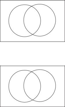
In the sum P (E)+P (F ) the weights of elements of E ∩F each appear twice, while the weights of all other elements of E F each appear once. We can see this by looking at a diagram called a Venn Diagram. In a Venn diagram, the rectangle represents the sample space, and the circles represent the events.

If we were to shade both E and F V, we would wind up shading the region E ∩ F twice. We represent that by putting numbers in the regions, representing how many times they are shaded.

This illustrates why the sum P (E) + P (F ) includes the weight of each element of E ∩ F twice. Thus to get a sum that includes the weight of each element of E F exactly once, we have to subtract the weight of E F from the sum P (E) + P (F ). This is why