

Discrete.Math.in.Computer.Science,2002
.pdf100 |
CHAPTER 4. INDUCTION, RECURSION AND RECURRENCES |
Thus by the principle of mathematical induction, there is a unique path between any two vertices in a rooted tree.
We have just proved the following.
Theorem 4.3.2 For each vertex x and y in a rooted tree, there is a unique path joining x to y.
Notice that in our inductive proof, we never mentioned of an integer n. There were integers there implicitly—the number of vertices in the whole tree and the number in each subtree are relevant—but it was unnecessary to mention them. Instead we simply used the fact that we were decomposing a structure (the tree) into smaller structures of the same type (the subtrees) as our inductive step and the fact that we could prove our result for the smallest substructures we could get to by decomposition (in this case, the single vertex trees) as our base case. It is clear that you could rewrite our proof to mention integers, and doing so would make it clear that mentioning them adds nothing to the proof. When we use mathematical induction in this way, using smaller structures in place of smaller integers, people say we are using structural induction.
In a rooted tree we refer to the nodes connected to the root as its children and we call the root their parent. We call the members of a subtree of r descendents of r, and we call r their ancestor. We use this language recursively throughout the tree. Thus in Figure 4.3 vertex x is a child of vertex z, but vertex x is not an ancestor of vertex y.
Graphs and trees
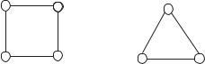
Our use of the phrase “rooted tree” suggests that there must be a concept of a unrooted tree or simply a tree. In fact there is such a concept; it is a special case of the idea of a graph. A graph consists of a set called a vertex set and another set called an edge set. While we don’t define exactly what we mean by vertices or edges, we do require that each edge is associated with two vertices that we call its endpoints. Walks and paths are defined in the same way they are for rooted trees. We draw pictures of graphs much as we would draw pictures of rooted trees (we just don’t have a special vertex that we draw at the ”top” of the drawing). In Figure 4.4 we show a typical drawing of a graph, and a typical drawing of a tree. What is a tree, though? A tree is a graph with property that there is a unique path between any two of its vertices. In Figure 4.4 we show an example of a graph that is not a tree (on the left) and a tree.
Figure 4.4: A graph and a tree.
Notice that the tree has ten vertices and nine edges. We can prove by induction that a tree on n vertices has n − 1 edges. The inductive proof could be modeled on the proof we used for
4.3. ROOTED TREES |
101 |
rooted trees, but it can also be done more simply, because deleting an edge and no vertices from a tree always gives us two trees (one has to think about the definition a bit to see this). We assume inductively that each of these trees has one fewer edge than vertex, so between them they have two fewer edges than vertices, so putting one edge back in completes the inductive step.
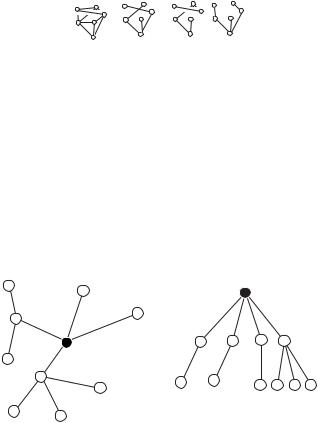
In computer science applications trees often arise in connection with graphs. For example the graph in Figure 4.5 might represent a communications network. If we want to send a message from the central vertex to each other vertex, we could choose a set of edges to send the message along. Each of the three trees in Figure 4.5 uses a minimum number of edges to send our message, so that if we have to pay for each edge we use, we pay a minimum amount to send our message. However if there is a time delay along each link (in military applications, for example, we might need to use a courier in times of radio silence), then the third tree might be preferred for sending messages from the center vertex to all other vertices. The three trees in Figure 4.5 are called spanning trees of our graph. A spanning tree of a graph is a tree that has the same vertex set as the graph and an edge set that is a subset of the edge set of the graph. As you might expect, there are many di erent criteria we might use for choosing a spanning tree of a graph.
Figure 4.5: Some spanning trees of a graph.
If it seems to you that there is not that much di erence between trees and rooted trees, you are right. We can conclude from what we have already shown that if you ignore the root of a rooted tree, you get a tree. (We showed that there is a unique path between any two vertices.) In fact, given a tree, we may choose any vertex and declare it to be a root, and we have a rooted tree. We illustrate the process in Figure 4.6. How would we prove this? One guess—induction!
Figure 4.6: Choosing a vertex in a tree to be a root gives us a rooted tree.
4.3-3 Show that deleting an edge from a tree gives us two trees.
4.3-4 Show that selecting a vertex in a tree gives a rooted tree according to our definition of a rooted tree.
102 |
CHAPTER 4. INDUCTION, RECURSION AND RECURRENCES |
For Exercise 4.3-3, suppose we have a tree which we call T . Remember by definition a tree is a graph with a unique path between any pair of vertices. Choose an edge with endpoints x and y in T . Every vertex that had a path to x that did not use the edge (x, y) still has a path to x and every vertex that had a path to y that did not use the edge (x, y) still has a path to y. If a vertex v has no path to either x or y after we have removed the edge, then putting the edge from x to y back in cannot create a path from v to either x or y. Therefore every vertex has a path to either x or y after the edge is deleted, so removing the edge has given us two graphs each that have a path between each pair of their points. Those paths must be unique because they were unique before we deleted the edge. Thus we get two trees.
To do Exercise 4.3-4, we begin by noting that a single vertex is both a tree and a rooted tree according to our two definitions. Now suppose that choosing a root in a tree with n − 1 or fewer vertices gives a tree, and let T stand for a tree on n vertices with n > 1. Choose a vertex y and an edge (x, y). Delete the edge. In the trees Tx and Ty that result, choose the vertices x and y to be roots, which, by our inductive hypothesis gives us rooted trees. Suppose the subtrees of the root y in the tree Ty are T1, T2, . . . , Tk . Let T be the tree with root vertex y and subtrees Tx, T1, T2, . . . , Tk The by our recursive definition, T is a rooted tree. Therefore, by the principle of mathematical induction, choosing a vertex to be root in any tree gives a rooted tree. Notice how little reference we actually made to the integer n. We could delete these references and simply make our inductive hypothesis for smaller trees and we would have a proof by structural induction.
This completes a proof of the following theorem.
Theorem 4.3.3 Any rooted tree is a tree, and choosing a vertex in a tree to call a root creates a rooted tree.
Connected and Disconnected graphs
The graph in Figure 4.7 looks like two graphs. It is called a disconnected graph. In contrast, the two graphs in Figure 4.4 are called connected graphs.
Figure 4.7: A disconnected graph.
1 |
2 |
6 |
4 |
3 |
5 |
7 |
|
|
A graph is called connected if for each x and y in the graph, there is a walk from x to y. The relation of being connected is an equivalence relation, because the relation partitions the vertex set into disjoint sets as follows: For each x, let
Sx = {y| x and y are connected by a walk.}
Then the sets Sx and Sy sets Sx form a partition
are either identical or disjoint, and each x is in Sx. Thus the distinct of the vertex set of the graph. The sets Sx are called the connected
4.3. ROOTED TREES |
103 |
components of the graph. A tree is connected because there is a path between any two of its vertices.
In Figure 4.7 the walks from 1 to 2 to 3 and back to 1 and from 1 to 2 to 3 to 4 and back to 1 are called cycles. A cycle is a walk whose first and last vertex are the same but has no other vertices or edges that are repeated.
4.3-5 Find the other cycles in Figure 4.7.
4.3-6 Can a tree have any cycles?
4.3-7 Is a connected graph with no cycles a tree?
The other cycles in Figure 4.7 are the walk from 1 to 3 to 4 and back to 1 and the walk from 5 to 6 to 7 and back to 5. Trees have no cycles and a graph is a tree if and only if it is connected and has no cycles.
Theorem 4.3.4 A graph G is a tree if and only if it is connected and has no cycles.
Proof: Suppose G is a tree. Then it is connected because between any two vertices there is a path. If G had a cycle, then we would use it to give two paths between any two vertices on the cycle, contradicting the definition of a tree. Therefore G has no cycles.
Suppose now that G is connected and has no cycles. Then there is a walk between any two vertices, so leaving out portions of the walk between successive repeated vertices, and continuing to do so until there are no repeated vertices will give give a path. Suppose now there are two distinct paths that start at the same vertex and end at the same vertex. Among all such pairs of paths, choose a pair with as few common vertices as possible. There must be at least two common vertices, the starting vertex s and the ending vertex t. If there were a third vertex x on both paths, then the portions of the two paths that go from s to x would two distinct paths with fewer common vertices or else would be identical, and the portions of the two paths that go from x to t would either be two distinct paths with fewer common vertices or would be identical. In any case, having such a vertex contradicts the assumption that we had a pair of distinct paths with as few common vertices as possible. Thus there is no such x. Therefore going from s to t on one path and then from t to s on the other gives a cycle, a contradiction to our hypothesis that G has no cycles. Thus the supposition of two distinct paths that start at the same and end at the same vertex is impossible, so G is a tree. 
Problems
1.Draw all rooted trees on 5 vertices. The order and the place in which you write the vertices down on the page is unimportant. If you would like to label the vertices (as we did in the graph in Figure 4.7), that is fine, but the way in which you assign labels to the vertices is unimportant.
2.A vertex of a rooted tree is called a leaf node if it has no children. Draw all rooted trees on 6 vertices with four leaf nodes.
104 |
CHAPTER 4. INDUCTION, RECURSION AND RECURRENCES |
3.Draw all di erent trees on six vertices. Two trees are not considered di erent if simply by redrawing one we get the other. In other words, if you can label the vertices so that when you write down for each edge the labels of the pair of vertices they connect, you get exactly the same collections of pairs, then they are the same. In “fancier” terminology, graphs with the labelling property we just described are isomorphic.
4.Find a tree that has the property that all the rooted trees you get by picking di erent vertices as roots are di erent as rooted trees. (Two rooted trees are the same (isomorphic), if they each have one vertex or if you can label them so that they have the same (labelled) root and the same (labelled) subtrees.)
5.A binary tree is a special kind of rooted tree that has some additional structure that makes it tremendously useful as a data structure. In order to describe the idea of a binary tree it is useful to think of a tree with no vertices, which we call the null tree or empty tree. Then we can recursively describe a binary tree as an empty tree, or a structure consisting of a root vertex, a binary tree called the left subtree of the root and a binary tree called the right subtree of the root. Then a single vertex is a binary tree with an empty right subtree and an empty left subtree. A rooted tree with two nodes can occur in two ways as a binary tree, either with a root and a left subtree consisting of one vertex or as a root and a right subtree consisting of one vertex. Draw all binary trees on four vertices in which the root node has an empty right child. Draw all binary trees on four vertices in which the root has a nonempty left child and a nonempty right child.
6.A(left, right) child of a vertex in a binary tree is the root of a (left, right) subtree of that vertex. A binary tree is a full binary tree if each vertex has either two nonempty children or two empty children (a vertex with two empty children is called a leaf.) Draw all full binary trees on seven vertices.
7.Are there any full binary trees (see Exercise 4.3-6) on an even number of vertices? Prove that what you say is correct.
8.The depth of a node in a rooted tree is defined to be the number of edges on the (unique) path to the root. A binary tree is complete if it is full (see Exercise 4.3-6) and all its leaves (see Exercise 4.3-6) have the same depth. How many nodes does a complete binary tree of depth 1 have? Depth 2? Depth d? (Proof required for depth d.)
9.The height of a rooted or binary tree with one vertex is 0; otherwise it is 1 plus the maximum of the heights of its subtrees. Based on Exercise 4.3-8, what is the minimum height of any binary tree on n nodes? (Please prove this.)
10.A binary tree is complete if it is full and all its leaves have the same depth (see Exercise 4.3-6 and Exercise 4.3-8). A vertex that is not a leaf vertex is called an internal vertex. What is the relationship between the number I of internal nodes and the number L of leaf nodes in a complete binary tree. A full binary tree? (Proof please.)
11.The internal path length of a binary tree is the sum, taken over all internal (see Exercise 4.3-10) vertices of the tree, of the depth of the vertex. The external path length of a binary tree is the sum, taken over all leaf vertices of the tree, of the depth of the vertex. Show that in a full binary tree with n internal vertices, internal path length i and external path length e, we have e = i + 2n.
4.3. ROOTED TREES |
105 |
12.Show that a graph is connected if and only if it has a spanning tree.
13.Show that a graph on n vertices is a tree if and only if it is connected and has n − 1 edges.
14.A graph with no cycles is called a forest. Show that if a forest has v vertices, e edges, and c connected components, then v = e + c.
15.Show that a graph on n vertices is a tree if and only if it has n −1 edges and has no cycles.
106 |
CHAPTER 4. INDUCTION, RECURSION AND RECURRENCES |
4.4Growth Rates of Solutions to Recurrences
Divide and Conquer Algorithms
One of the most basic and powerful algorithmic techniques is divide and conquer. Consider, for example, the binary search algorithm, which we will describe in the context of guessing a number between 1 and 100. Suppose someone picks a number between 1 and 100, and allows you to ask questions of the form ”Is the number greater than k?” where k is an integer you choose. Your goal is to ask as few questions as possible to figure out the number. Your first question should be ”Is the number greater than 50?” Why is this? Well, after asking if the number is bigger than 50, you have learned either that the number is between one and 50, or that the number is between 51 and 100. In either case have reduced your problem to one in which the range is only half as big. Thus you have divided the problem up into a problem that is only half as big, and you can now (recursively) conquer this remaining problem. (If you ask any other question, one of the possible ranges of values you could end up with would more than half the size of the original problem.) If you continue in this fashion, always cutting the problem size in half, you will be able to get the problem down to size one fairly quickly, and then you will know what the number is. Of course it would be easier to cut the problem exactly in half each time if we started with a number in the range from one to 128, but the question doesn’t sound quite so plausible then. Thus to analyze the problem we will assume someone asks you to figure out a number between 0 and n, where n is a power of 2.
4.4-1 Let T (n) be number of questions in binary search on the range of numbers between 1 and n. Assuming that n is a power of 2, get a recurrence of for T (n).
For Exercise 4.4-1 we get:
T (n) = |
T (n/2) + 1 |
if n ≥ 2 |
(4.12) |
|
1 |
if n = 1 |
|
That is, the number of guesses to carry out binary search on n items is equal to 1 step (the guess) plus the time to solve binary search on the remaining n/2 items.
What we are really interested in is how much time it takes to use binary search in a computer program that looks for an item in an ordered list. While the number of questions gives us a feel for the amount of time, processing each question may take several steps in our computer program. The exact amount of time these steps take might depend on some factors we have little control over, such as where portions of the list are stored. Also, we may have to deal with lists whose length is not a power of two. Thus a more realistic description of the time needed would be
T (n) |
≤ |
T ( n/2 ) + C1 |
if n ≥ 2 |
(4.13) |
|
C2 |
if n = 1, |
|
where C1 and C2 are constants.
It turns out that the solution to (4.12) and (4.13) are roughly the same, in a sense that will hopefully become clear later in the notes. This is almost always the case; we will come back to

4.4. GROWTH RATES OF SOLUTIONS TO RECURRENCES |
107 |
this issue. For now, let us not worry about floors and ceilings and the distinction between things that take 1 unit of time and things that take no more than some constant amount of time.
Let’s turn to another example of a divide and conquer algorithm, mergesort. In this algorithm, you wish to sort a list of n items. Let us assume that the data is stored in an array A in positions 1 through n. Mergesort can be described as follows:
MergeSort(A,low,high)
if (low == high)
return
else
mid = (low + high) /2 MergeSort(A,low,mid) MergeSort(A,mid+1,high)
Merge the sorted lists from the previous two steps
More details on mergesort can be found in almost any algorithms textbook. Su ce to say that the base case (low = high) takes one step, while the other case executes 1 step, makes two recursive calls on problems of size n/2, and then executes the Merge instruction, which can be done in n steps.
Thus we obtain the following recurrence for the running time of mergesort:
T (n) = |
2T (n/2) + n if n > 1 |
(4.14) |
||
1 |
if n = 1 |
|||
|
|
|||
Recurrences such as this one can be understood via the idea of a recursion tree, which we introduce below. This concept will allow us to analyze recurrences that arise in divide-and- conquer algorithms, and those that arise in other recursive situations, such as the Towers of Hanoi, as well.
Recursion Trees
We will introduce the idea of a recursion tree via several examples. It is helpful to have an “algorithmic” interpretation of a recurrence. For example, (ignoring for a moment the base case) we can interpret the recurrence
T (n) = 2T (n/2) + n |
(4.15) |
as “in order to solve a problem of size n we must solve 2 problems of size n/2 and do n units of additional work.” Similarly we can interpret
T (n) = T (n/4) + n2
as “in order to solve a problem of size n we must solve 1 problems of size n/4 and do n2 units of additional work.”
We can also interpret the recurrence
T (n) = 3T (n − 1) + n
108 |
CHAPTER 4. INDUCTION, RECURSION AND RECURRENCES |
as “in order to solve a problem of size n, we must solve 3 subproblems of size n − 1 and do n additional units of work.
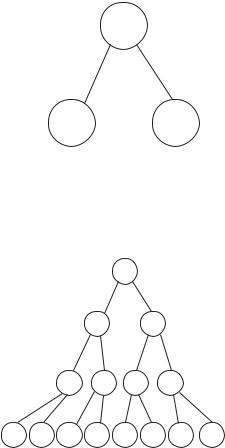
We will now draw the beginning of the recursion diagram for (4.15). For now, assume n is a power of 2. A recursion tree diagram has three parts. On the left, we keep track of the problem size, in the middle we draw the tree, and on right we keep track of the work done. So to begin the recursion tree for (4.15), we take a problem of size n, split it into 2 problems of size n/2 and note on the right that we do n units of work. The fact that we break the problem into 2 problems is denoted by drawing two children of the root node (level 0). This gives us the following picture.
Problem Size |
Work |
n |
n |
n/2
We then continue to draw the tree in this manner. Adding a few more levels, we have:
Problem Size |
Work |
n |
n |
n/2 |
n/2 + n/2 = n |
|
|
n/4 |
n/4 + n/4 + n/4 + n/4 = n |
n/8 |
8(n/8) = n |
At level zero (the top level), n units of work are done. We see that at each succeeding level, we halve the problem size and double the number of subproblems. We also see that at level 1, each of the two subproblems requires n/2 units of additional work, and so a total of n units of additional work are done. Similarly the second level has 4 subproblems of size n/4 and so 4(n/4) units of additional work are done.
We now have enough information to be able to describe the recursion tree diagram in general. To do this, we need to determine, for each level i, three things
4.4. GROWTH RATES OF SOLUTIONS TO RECURRENCES |
109 |
•number of subproblems,
•size of each subproblem,
•total work done.
We also need to figure out how many levels there are in the recursion tree.
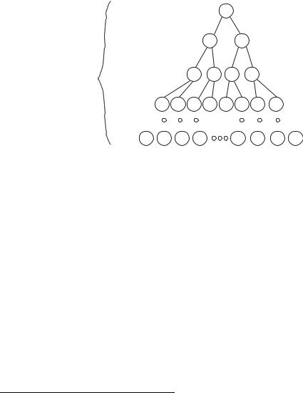
We see that for this problem, at level i, we have 2i subproblems of size n/2i. Further, since a problem of size 2i requires 2i units of additional work, there are (2i)[n/(2i)] = n units of work done per level. To figure out how many levels there are in the tree, we just notice that at each level the problem size is cut in half, and the tree stops when the problem size is 1. Therefore there are log2 n + 1 levels of the tree, since we start with the top level and cut the problem size in half log2 n times.1 We can thus visualize the whole tree as follows:
Problem Size |
Work |
n |
n |
n/2 |
n/2 + n/2 = n |
|
|
log n +1 |
|
levels |
|
n/4 |
n/4 + n/4 + n/4 + n/4 = n |
n/8 |
8(n/8) = n |
1 |
n(1) = n |
The bottom level is di erent from the other levels. In the other levels, the work is described by the recursive part of the recurrence, which in this case is T (n) = 2T (n/2) + n. At the bottom level, the work comes from the base case. Thus we must compute the number of problems of size 1 (assuming that one is the base case), and then multiply this value by T (1). For this particular recurrence, and for many others, it turns out that if you compute the amount of work on the bottom level as if you were computing the amount of additional work required after you split a problem of size one into 2 problems (which, of course, makes no sense) it will be the same value as if you compute it via the base case. We emphasize that the correct value always comes from the base case, it is just a useful coincidence that it sometimes also comes from the recursive part of the recurrence.
The important thing is that we now know exactly how many levels there are, and how much work is done at each level. Once we know this, we can sum the total amount of work done over all the levels, giving us the solution to our recurrence. In this case, there are log2 n + 1 levels, and at each level the amount of work we do is n units. Thus we conclude that the total amount of work done to solve the problem described by recurrence (4.15) is n(log2 n + 1). The total work done throughout the tree is the solution to our recurrence, because the tree simply models the process of iterating the recurrence. Thus the solution to recurrence (4.14) is T (n) = n(log n + 1).
1To simplify notation, for the remainder of the book, if we omit the base of a logarithm, it should be assumed to be base 2.