CP = Cp x M

where Cp is the specific heat capacity of the stream (KJ/ºC, kg) and M is the mass flowrate (kg/sec). The CP of a stream is measured as enthalpy change per unit temperature (kW/ºC or equivalent units). For this example a minimum temperature difference of 10ºC is assumed during the analysis which is the same as in the existing process, as highlighted in the Data Extraction Flowsheet. The hot utility is steam available at 200ºC and the cold utility is cooling water available between 25ºC to 30ºC.

1.4 Energy Targets

Starting from the thermal data for a process (such as shown in the thermal analysis table), Pinch Analysis provides a target for the minimum energy consumption. The energy targets are obtained using a tool called the "Composite Curves".

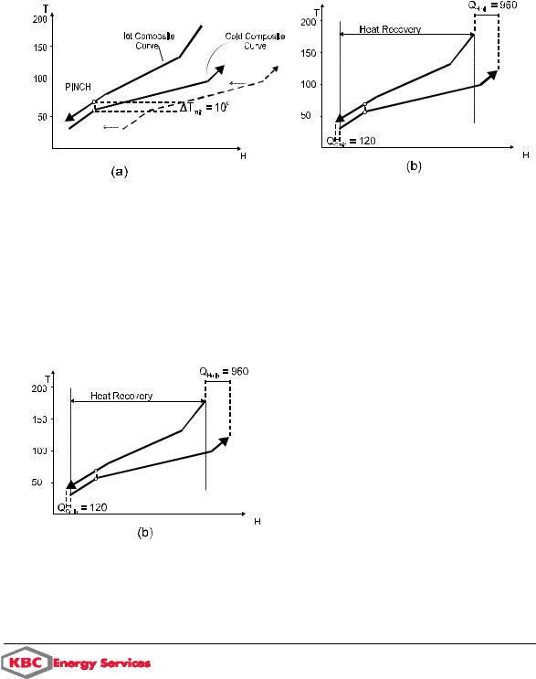
1.4.1 Construction of Composite Curves

Composite Curves consist of temperature-enthalpy (T-H) profiles of heat availability in the process (the "hot composite curve") and heat demands in the process (the "cold composite curve") together in a graphical representation. The figure below illustrates the construction of the "hot composite curve" for the example process, which has two hot streams (stream number 1 and 2, see the thermal analysis table). Their T-H representation is shown in Figure

(a) and their composite representation is shown in Figure (b). Stream 1 has a CP of 20 kW/°C, and is cooled from 180°C to 80°C, releasing 2000kW of heat. Stream 2 is cooled from 130°C to 40°C and with a CP of 40kW/°C and loses 3600kW.

Construction of Composite Curves

The construction of the hot composite curve (as shown in Figure (b)) simply involves the addition of the enthalpy changes of the streams in the respective temperature intervals. In the temperature interval 180ºC to 130ºC only stream 1 is present. Therefore the CP of the composite curve equals the CP of stream 1 i.e. 20. In the temperature interval 130ºC to 80ºC, both streams 1 and 2 are present, therefore the CP of the hot composite equals the sum of the CP's of the two streams i.e. 20+40=60. In the temperature interval 80ºC to 40ºC only

Pinch Technology Introduction

stream 2 is present, thus the CP of the composite is 40. The construction of the cold composite curve is similar to that of the hot composite curve involving the combination of the cold stream T-H curves for the process.

1.4.2 Determining the Energy Targets

The composite curves provide a counter-current picture of heat transfer and can be used to indicate the minimum energy target for the process. This is achieved by overlapping the hot and cold composite curves, as shown in Figure (a), separating them by the minimum temperature difference DTmin (10ºC for the example process). This overlap shows the maximum process heat recovery possible (Figure (b)), indicating that the remaining heating and cooling needs are the minimum hot utility requirement (QHmin) and the minimum cold utility requirement (QCmin ) of the process for the chosen DTmin.

Using the hot and cold composite curves to determine the energy targets

The composite curves in the figure above have been constructed for the example process (Click here for the Data Extraction Flowsheet or the thermal analysis table). The minimum hot utility (QHmin) for the example problem is 960 units which is less than the existing process energy consumption of 1200 units. The potential for energy saving is therefore 1200-960 = 240 units by using the same value of DTmin as the existing process. Using Pinch Analysis, targets for minimum energy consumption can be set purely on the basis of heat and material balance information, prior to heat exchanger network design. This allows quick identification of the scope for energy saving at an early stage.

1.4.4 The Pinch Principle

The point where DTmin is observed is known as the "Pinch" and recognising its implications allows energy targets to be realised in practice. Once the pinch has been identified, it is possible to consider the process as two separate systems: one above and one below the pinch, as shown in Figure (a). The system above the pinch requires a heat input and is therefore a net heat sink. Below the pinch, the system rejects heat and so is a net heat source.

The Pinch Principle

In Figure (b), α amount of heat is transferred from above the pinch to below the pinch. The system above the pinch, which was before in heat balance with QHmin, now loses α units of heat to the system below the pinch. To restore the heat balance, the hot utility must be increased by the same amount, that is, α units. Below the pinch, α units of heat are added to the system that had an excess of heat, therefore the cold utility requirement also increases by α units. In conclusion, the consequence of a cross-pinch heat transfer (α) is that both the hot and cold utility will increase by the cross-pinch duty (α).

For the example process (click for the flowsheet, or Composite Curves) the cross pinch heat transfer in the existing process is equal to 1200-960 = 240 units.

Figure (b) also shows γ amount of external cooling above the pinch and β amount of external heating below the pinch. The external cooling above the pinch of γ amount increases the hot utility demand by the same amount. Therefore on an overall basis both the hot and cold utilities are increased by γ amount. Similarly external heating below the pinch of β amount increases the overall hot and cold utility requirement by the same amount (i.e. β).

To summarise, the understanding of the pinch gives three rules that must be obeyed in order to achieve the minimum energy targets for a process:

•Heat must not be transferred across the pinch

•There must be no external cooling above the pinch

•There must be no external heating below the pinch

Violating any of these rules will lead to cross-pinch heat transfer resulting in an increase in the energy requirement beyond the target. The rules form the basis for the network design

Pinch Technology Introduction