

B.Crowell - Vibrations and Waves, Vol
.3.pdfTop: A series of images from a silent movie of the bridge vibrating on the day it was to collapse, taken by an unknown amateur photographer.
Middle: The bridge immediately before the collapse, with the sides vibrating 8.5 meters (28 feet) up and down. Note that the bridge is over a mile long.
Bottom: During and after the final collapse. The right-hand picture gives a sense of the massive scale of the construction.
2 Resonance
Soon after the mile-long Tacoma Narrows Bridge opened in July 1940, motorists began to notice its tendency to vibrate frighteningly in even a moderate wind. Nicknamed “Galloping Gertie,” the bridge collapsed in a steady 42-mile-per-hour wind on November 7 of the same year. The following is an eyewitness report from a newspaper editor who found himself on the bridge as the vibrations approached the breaking point.
“Just as I drove past the towers, the bridge began to sway violently from side to side. Before I realized it, the tilt became so violent that I lost control of the car... I jammed on the brakes and got out, only to be thrown onto my face against the curb.
“Around me I could hear concrete cracking. I started to get my dog Tubby, but was thrown again before I could reach the car. The car itself began to slide from side to side of the roadway.
“On hands and knees most of the time, I crawled 500 yards or more to the towers... My breath was coming in gasps; my knees were raw and bleeding, my hands bruised and swollen from gripping the concrete curb...
Toward the last, I risked rising to my feet and running a few yards at a time... Safely back at the toll plaza, I saw the bridge in its final collapse and
Section 21

saw my car plunge into the Narrows.”
The ruins of the bridge formed an artificial reef, one of the world’s largest. It was not replaced for ten years. The reason for its collapse was not substandard materials or construction, nor was the bridge underdesigned: the piers were hundred-foot blocks of concrete, the girders massive and made of carbon steel. The bridge was destroyed because of the physical phenomenon of resonance, the same effect that allows an opera singer to break a wine glass with her voice and that lets you tune in the radio station you want. The replacement bridge, which has lasted half a century so far, was built smarter, not stronger. The engineers learned their lesson and simply included some slight modifications to avoid the resonance phenomenon that spelled the doom of the first one.
2.1 Energy in Vibrations
One way of describing the collapse of the bridge is that the bridge kept taking energy from the steadily blowing wind and building up more and more energetic vibrations. In this section, we discuss the energy contained in a vibration, and in the subsequent sections we will move on to the loss of energy and the adding of energy to a vibrating system, all with the goal of understanding the important phenomenon of resonance.
Going back to our standard example of a mass on a spring, we find that there are two forms of energy involved: the potential energy stored in the spring and the kinetic energy of the moving mass. We may start the system in motion either by hitting the mass to put in kinetic energy by pulling it to one side to put in potential energy. Either way, the subsequent behavior of the system is identical. It trades energy back and forth between kinetic and potential energy. (We are still assuming there is no friction, so that no energy is converted to heat, and the system never runs down.)
The most important thing to understand about the energy content of vibrations is that the total energy is proportional to the square of the amplitude. Although the total energy is constant, it is instructive to consider two specific moments in the motion of the mass on a spring as examples. When the mass is all the way to one side, at rest and ready to reverse directions, all its energy is potential. We have already seen that the
potential energy stored in a spring equals 12kx 2 , so the energy is propor-
tional to the square of the amplitude. Now consider the moment when the mass is passing through the equilibrium point at x=0. At this point it has no potential energy, but it does have kinetic energy. The velocity is propor-
tional to the amplitude of the motion, and the kinetic energy, 12mv 2 , is
proportional to the square of the velocity, so again we find that the energy is proportional to the square of the amplitude. The reason for singling out these two points is merely instructive; proving that energy is proportional to A2 at any point would suffice to prove that energy is proportional to A2 in general, since the energy is constant.
Are these conclusions restricted to the mass-on-a-spring example? No. We have already seen that F=–kx is a valid approximation for any vibrating object, as long as the amplitude is small. We are thus left with a very general
22 |
Chapter 2 Resonance |
conclusion: the energy of any vibration is approximately proportional to the square of the amplitude, provided that the amplitude is small.
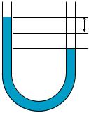
Example: water in a U-tube
If water is poured into a U-shaped tube as shown in the figure, it can undergo vibrations about equilibrium. The energy of such a vibration is most easily calculated by considering the “turnaround
A point” when the water has stopped and is about to reverse directions. At this point, it has only potential energy and no kinetic energy, so by calculatings its potential energy we can find the energy of the vibration. This potential energy is the same as the work that would have to be done to take the water out of the right-hand side down to a depth A below the equilibrium level, raise it through a height A, and place it in the left-hand side. The weight of this chunk of water is proportional to A, and so is the height through which it must be lifted, so the energy is proportional to A2.
Example: the range of energies of sound waves
Question: The amplitude of vibration of your eardrum at the threshold of pain is about 106 times greater than the amplitude with which it vibrates in response to the softest sound you can hear. How many times greater is the energy with which your ear has to cope for the painfully loud sound, compared to the soft sound?
Solution: The amplitude is 106 times greater, and energy is proportional to the square of the amplitude, so the energy is greater by a factor of 1012. This is a phenomenally large factor!
We are only studying vibrations right now, not waves, so we are not yet concerned with how a sound wave works, or how the energy gets to us through the air. Note that because of the huge range of energies that our ear can sense, it would not be reasonable to have a sense of loudness that was additive. Consider, for instance, the following three levels of sound:
barely audible, gentle wind |
|
quiet conversation ..................... |
105 times more energy than the wind |
heavy metal concert................... |
1012 times more energy than the wind |
In terms of addition and subtraction, the difference between the wind and the quiet conversation is nothing compared to the difference between the quiet conversation and the heavy metal concert. Evolution wanted our sense of hearing to be able to encompass all these sounds without collapsing the bottom of the scale so that anything softer than the crack of doom would sound the same. So rather than making our sense of loudness additive, mother nature made it multiplicative. We sense the difference between the wind and the quiet conversation as spanning a range of about 5/12 as much as the whole range from the wind to the heavy metal concert. Although a detailed discussion of the decibel scale is not relevant here, the basic point to note about the decibel scale is that it is logarithmic. The zero of the decibel scale is close to the lower limit of human hearing, and adding 1 unit to the decibel measurement corresponds to multiplying the energy level (or actually the power per unit area) by a certain factor.
Section 2.1 Energy in Vibrations |
23 |
2.2 Energy Lost From Vibrations
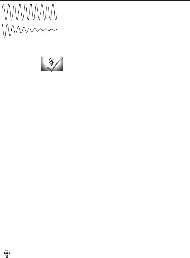
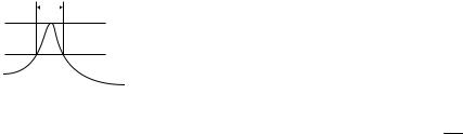
Friction has the effect of pinching the x-t graph of a vibrating object.
Until now, we have been making the relatively unrealistic assumption that a vibration would never die out. For a realistic mass on a spring, there will be friction, and the kinetic and potential energy of the vibrations will therefore be gradually converted into heat. Similarly, a guitar string will slowly convert its kinetic and potential energy into sound. In all cases, the effect is to “pinch” the sinusoidal x-t graph more and more with passing time. Friction is not necessarily bad in this context — a musical instrument that never got rid of any of its energy would be completely silent! The dissipation of the energy in a vibration is known as damping.
Most people who try to draw graphs like those shown on the left will tend to shrink their wiggles horizontally as well as vertically. Why is this wrong?
In the graphs on the left, I have not shown any point at which the damped vibration finally stops completely. Is this realistic? Yes and no. If energy is being lost due to friction between two solid surfaces, then we expect the force of friction to be nearly independent of velocity. This constant friction force puts an upper limit on the total distance that the vibrating object can ever travel without replenishing its energy, since work equals force times distance, and the object must stop doing work when its energy is all converted into heat. (The friction force does reverse directions when the object turns around, but reversing the direction of the motion at the same time that we reverse the direction of the force makes it certain that the object is always doing positive work, not negative work.)
Damping due to a constant friction force is not the only possibility however, or even the most common one. A pendulum may be damped mainly by air friction, which is approximately proportional to v2, while other systems may exhibit friction forces that are proportional to v. It turns out that friction proportional to v is the simplest case to analyze mathematically, and anyhow all the important physical insights can be gained by studying this case.
If the friction force is proportional to v, then as the vibrations die down, the frictional forces get weaker due to the lower speeds. The less energy is left in the system, the more miserly the system becomes with giving away any more energy. Under these conditions, the vibrations theoretically never die out completely, and mathematically, the loss of energy from the system is exponential: the system loses a fixed percentage of its energy per cycle. This is referred to as exponential decay.
A nonrigorous proof is as follows. The force of friction is proportional to v, and v is proportional to how far the objects travels in one cycle, so the frictional force is proportional to amplitude. The amount of work done by friction is proportional to the force and to the distance traveled, so the work done in one cycle is proportional to the square of the amplitude. Since both the work and the energy are proportional to A2, the amount of energy taken away by friction in one cycle is a fixed percentage of the amount of energy the system has.
The horizontal axis is a time axis, and the period of the vibrations is independent of amplitude. Shrinking the amplitude does not make the cycles any faster.
24 |
Chapter 2 Resonance |
Self-Check
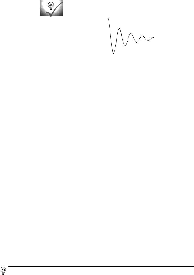
The figure shows an x-t graph for a strongly damped vibration, which loses half of its amplitude with every cycle. What fraction of the energy is lost in each cycle?
It is customary to describe the amount of damping with a quantity called the quality factor, Q, defined as the number of cycles required for the energy to fall off by a factor of 535. (The origin of this obscure numerical factor is e2π, where e=2.71828... is the base of natural logarithms.) The terminology arises from the fact that friction is often considered a bad thing, so a mechanical device that can vibrate for many oscillations before it loses a significant fraction of its energy would be considered a high-quality device.
Example: exponential decay in a trumpet
Question: The vibrations of the air column inside a trumpet have a Q of about 10. This means that even after the trumpet player stops blowing, the note will keep sounding for a short time. If the player suddenly stops blowing, how will the sound intensity 20 cycles later compare with the sound intensity while she was still blowing?
Solution: The trumpet’s Q is 10, so after 10 cycles the energy will have fallen off by a factor of 535. After another 10 cycles we lose another factor of 535, so the sound intensity is reduced by a factor of 535x535=2.9x10⁵.
The decay of a musical sound is part of what gives it its character, and a good musical instrument should have the right Q, but the Q that is considered desirable is different for different instruments. A guitar is meant to keep on sounding for a long time after a string has been plucked, and might have a Q of 1000 or 10000. One of the reasons why a cheap synthesizer sounds so bad is that the sound suddenly cuts off after a key is released.
Example: Q of a stereo speaker
Stereo speakers are not supposed to reverberate or “ring” after an electrical signal that stops suddenly. After all, the recorded music was made by musicians who knew how to shape the decays of their notes correctly. Adding a longer “tail” on every note would make it sound wrong. We therefore expect that stereo speaker will have a very low Q, and indeed, most speakers are designed with a Q of about 1. (Low-quality speakers with larger Q values are referred to as “boomy.”)
We will see later in the chapter that there are other reasons why a speaker should not have a high Q.
Energy is proportional to the square of amplitude, so its energy is four times smaller after every cycle. It loses three quarters of its energy with each cycle.
Section 2.2 Energy Lost From Vibrations |
25 |
2.3 |
|
Putting Energy Into Vibrations |
||||
x |
|
|
|
|
When pushing a child on a swing, you cannot just apply a constant |
|
|
|
|
|
force. A constant force will move the swing out to a certain angle, but will |
||
|
|
|
|
|||
(a) |
|
|
|
t |
not allow the swing to start swinging. Nor can you give short pushes at |
|
|
|
|
randomly chosen times. That type of random pushing would increase the |
|||
|
|
|
|
|
|
|
F |
|
|
|
|
child’s kinetic energy whenever you happened to be pushing in the same |
|
|
|
|
|
|||
|
|
|
|
direction as her motion, but it would reduce her energy when your pushing |
||
|
|
|
|
|||
(b) |
|
|
|
t |
happened to be in the opposite direction compared to her motion. To make |
|
|
|
|
her build up her energy, you need to make your pushes rhythmic, pushing |
|||
|
|
|
|
|
|
|
F |
|
|
|
|
at the same point in each cycle. In other words, your force needs to form a |
|
|
|
|
|
|||
|
|
|
|
repeating pattern with the same frequency as the normal frequency of |
||
|
|
|
|
|||
(c) |
|
|
|
t |
vibration of the swing. Graph (a) shows what the child’s x-t graph would |
|
|
|
|
|
|
look like as you gradually put more and more energy into her vibrations. A |
|
|
|
|
|
|
|
|
|
|
|
|
|
|
graph of your force versus time would probably look something like graph |
|
|
|
|
|
|
|
|
|
|
|
|
|
(b). It turns out, however, that it is much simpler mathematically to |
|
|
|
|
|
|
consider a vibration with energy being pumped into it by a driving force |
|
|
|
|
|
|
that is itself a sine-wave, (c). A good example of this is your eardrum being |
|
|
|
|
|
|
driven by the force of a sound wave. |
|
|
|
|
|
|
Now we know realistically that the child on the swing will not keep |
|
|
|
|
|
|
increasing her energy forever, nor does your eardrum end up exploding |
|
|
|
|
|
|
because a continuing sound wave keeps pumping more and more energy |
|
|
|
|
|
|
into it. In any realistic system, there is energy going out as well as in. As the |
|
|
|
|
|
|
vibrations increase in amplitude, there is an increase in the amount of |
|
|
|
|
|
|
energy taken away by damping with each cycle. This occurs for two reasons. |
x |
|
|
|
|
Work equals force times distance (or, more accurately, the area under the |
|
|
|
|
|
force-distance curve). As the amplitude of the vibrations increases, the |
||
|
|
|
|
|
|
|
(d) |
|
|
t |
|
damping force is being applied over a longer distance. Furthermore, the |
|
|
|
|
damping force usually increases with velocity (we usually assume for |
|||
|
|
|
|
|
|
|
|
|
|
|
|
|
simplicity that it is proportional to velocity), and this also serves to increase |
|
|
|
|
|
|
|
|
|
|
|
|
|
the rate at which damping forces remove energy as the amplitude increases. |
|
|
|
|
|
|
Eventually (and small children and our eardrums are thankful for this!), the |
|
|
|
|
|
|
amplitude approaches a maximum value (d) at which energy is removed by |
|
|
|
|
|
|
the damping force just as quickly as it is being put in by the driving force. |
|
|
|
|
|
|
This process of approaching a maximum amplitude happens extremely |
|
|
|
|
|
|
quickly in many cases, e.g. the ear or a radio receiver, and we don’t even |
|
|
|
|
|
|
notice that it took a millisecond or a microsecond for the vibrations to |
|
|
|
|
|
|
“build up steam.” We are therefore mainly interested in predicting the |
|
|
|
|
|
|
behavior of the system once it has had enough time to reach essentially its |
|
|
|
|
|
|
maximum amplitude. This is known as the steady-state behavior of a |
|
|
|
|
|
|
vibrating system. |
|
|
|
|
|
|
Now comes the interesting part: what happens if the frequency of the |
|
|
|
|
|
|
driving force is mismatched to the frequency at which the system would |
|
|
|
|
|
|
naturally vibrate on its own? We all know that a radio station doesn’t have |
|
|
|
|
|
|
to be tuned in exactly, although there is only a small range over which a |
|
|
|
|
|
|
given station can be received. The designers of the radio had to make the |
26 |
Chapter 2 Resonance |
range fairly small to make it possible eliminate unwanted stations that happened to be nearby in frequency, but it couldn’t be too small or you wouldn’t be able to adjust the knob accurately enough. (Even a digital radio can be tuned to 88.0 MHz and still bring in a station at 88.1 MHz.) The ear also has some natural frequency of vibration, but in this case the range of frequencies to which it can respond is quite broad. Evolution has made the ear’s frequency response as broad as possible because it was to our ancestors’ advantage to be able to hear everything from a low roars to a high-pitched shriek.
The remainder of this section develops four important facts about the response of a system to a driving force whose frequency is not necessarily the same is the system’s natural frequency of vibration. The style is approximate and intuitive, but proofs are given in the subsequent optional section.
First, although we know the ear has a frequency — about 4000 Hz — at which it would vibrate naturally, it does not vibrate at 4000 Hz in response to a low-pitched 200 Hz tone. It always responds at the frequency at which it is driven. Otherwise all pitches would sound like 4000 Hz to us. This is a general fact about driven vibrations:
(1) The steady-state response to a sinusoidal driving force occurs at the frequency of the force, not at the system’s own natural frequency of vibration.
Now let’s think about the amplitude of the steady-state response. Imagine that a child on a swing has a natural frequency of vibration of 1 Hz, but we are going to try to make her swing back and forth at 3 Hz. We intuitively realize that quite a large force would be needed to achieve an amplitude of even 30 cm, i.e. the amplitude is less in proportion to the force. When we push at the natural frequency of 1 Hz, we are essentially just pumping energy back into the system to compensate for the loss of energy due to the damping (friction) force. At 3 Hz, however, we are not just counteracting friction. We are also providing an extra force to make the child’s momentum reverse itself more rapidly than it would if gravity and the tension in the chain were the only forces acting. It is as if we are artificially increasing the k of the swing, but this is wasted effort because we spend just as much time decelerating the child (taking energy out of the system) as accelerating her (putting energy in).
Now imagine the case in which we drive the child at a very low frequency, say 0.02 Hz or about one vibration per minute. We are essentially just holding the child in position while very slowly walking back and forth. Again we intuitively recognize that the amplitude will be very small in proportion to our driving force. Imagine how hard it would be to hold the child at our own head-level when she is at the end of her swing! As in the too-fast 3 Hz case, we are spending most of our effort in artificially changing the k of the swing, but now rather than reinforcing the gravity and tension forces we are working against them, effectively reducing k. Only a very small part of our force goes into counteracting friction, and the rest is used in repetitively putting potential energy in on the upswing and taking it back out on the downswing, without any long-term gain.
We can now generalize to make the following statement, which is true for all driven vibrations:
Section 2.3 Putting Energy Into Vibrations |
27 |

(2) A vibrating system resonates at its own natural frequency. That is, the amplitude of the steady-state response is greatest in proportion to the amount of driving force when the driving force matches the natural frequency of vibration.
The collapsed section of the Nimitz Freeway.
28 |
Chapter 2 Resonance |
Example: an opera singer breaking a wineglass
In order to break a wineglass by singing, an opera singer must first tap the glass to find its natural frequency of vibration, and then sing the same note back.
Example: collapse of the Nimitz Freeway in an earthquake
I led off the chapter with the dramatic collapse of the Tacoma Narrows Bridge, mainly because a it was well documented by a local physics professor, and an unknown person made a movie of the collapse. The collapse a section of the Nimitz Freeway in Oakland, CA, during a 1989 earthquake is however a simpler example to analyze.
An earthquake consists of many low-frequency vibrations that occur simultaneously, which is why it sounds like a rumble of indeterminate pitch rather than a low hum. The frequencies that we can hear are not even the strongest ones; most of the energy is in the form of vibrations in the range of frequencies from about 1 Hz to 10 Hz.
Now all the structures we build are resting on geological layers of dirt, mud, sand, or rock. When an earthquake wave comes along, the topmost layer acts like a system with a certain natural frequency of vibration, sort of like a cube of jello on a plate being shaken from side to side. The resonant frequency of the layer depends on how stiff it is and also on how deep it is. The ill-fated section of the Nimitz freeway was built on a layer of mud, and analysis by geologist Susan E. Hough of the U.S. Geological Survey shows that the mud layer’s resonance was centered on about 2.5 Hz, and had a width covering a range from about 1 Hz to 4 Hz.
When the earthquake wave came along with its mixture of frequencies, the mud responded strongly to those that were close to its own natural 2.5 Hz frequency. Unfortunately, an engineering analysis after the quake showed that the overpass itself had a resonant frequency of 2.5 Hz as well! The mud responded strongly to the earthquake waves with frequencies close to 2.5 Hz, and the bridge responded strongly to the 2.5 Hz vibrations of the mud, causing sections of it to collapse.
Example: Collapse of the Tacoma Narrows Bridge
Let’s now examine the more conceptually difficult case of the Tacoma Narrows Bridge. The surprise here is that the wind was steady. If the wind was blowing at constant velocity, why did it shake the bridge back and forth? The answer is that once the bridge started twisting a little, it began acting like a kite or an airplane wing. It established swirling patterns of air flow around itself, of the kind that you can see in a moving cloud of smoke. Thus even though the wind velocity measured far away from any structures was constant, the bridge’s vibration at its own natural frequency of 0.2 Hz set up an alternating pattern of wind gusts in the air immediately around it, which then increased the amplitude of the bridge’s vibrations. This vicious cycle fed upon itself, increasing the amplitude of the vibrations until the bridge finally collapsed.
As long as we’re on the subject of collapsing bridges, it is worth bringing up the reports of bridges falling down when soldiers marching over them happened to step in rhythm with the bridge’s natural frequency of oscillation. This is supposed to have happened in 1831 in Manchester, England, and again in 1849 in Anjou, France. Many modern engineers and scientists, however, are suspicious of the analysis of these reports. It is possible that the collapses had more to do with poor construction and overloading than with resonance. The Nimitz Freeway and Tacoma Narrows Bridge are far better documented, and occurred in an era when engineers’ abilities to analyze the vibrations of a complex structure were much more advanced.
Example: emission and absorption of light waves by atoms
In a very thin gas, the atoms are sufficiently far apart that they can act as individual vibrating systems. Although the vibrations are of a very strange and abstract type described by the theory of quantum mechanics, they nevertheless obey the same basic rules as ordinary mechanical vibrations. When a thin gas made of a certain element is heated, it emits light waves with certain specific frequencies, which are like a fingerprint of that element. As with all other vibrations, these atomic vibrations respond most strongly to a driving force that matches their own natural frequency. Thus if we have a relatively cold gas with light waves of various frequencies passing through it, the gas will absorb light at precisely those frequencies at which it would emit light if heated.
(3) When a system is driven at resonance, the steady-state vibrations have an amplitude that is proportional to Q.
This is fairly intuitive. The steady-state behavior is an equilibrium between energy input from the driving force and energy loss due to damping. A low-Q oscillator, i.e. one with strong damping, dumps its energy faster, resulting in lower-amplitude steady-state motion.
Self-Check
If an opera singer is shopping for a wine glass that she can impress her friends by breaking, what should she look for?
Example: Piano strings ringing in sympathy with a sung note
Question: A sufficiently loud musical note sung near a piano with the lid raised can cause the corresponding strings in the piano to vibrate. (A piano has a set of three strings for each note, all struck by the same hammer.) Why would this trick be unlikely to work with a violin?
Solution: If you have heard the sound of a violin being plucked (the pizzicato effect), you know that the note dies away very quickly. In other words, a violin’s Q is much lower than a piano’s. This means that its resonances are much weaker in amplitude.
She should tap the wineglasses she finds in the store and look for one with a high Q, i.e. one whose vibrations die out very slowly. The one with the highest Q will have the highest-amplitude response to her driving force, making it more likely to break.
Section 2.3 Putting Energy Into Vibrations |
29 |
|
FWHM |
|||
energy of |
|
|
max. |
|
|
|
|||
steady- |
|
|
|
|
state |
|
|
1/2 max. |
|
vibrations |
|
|
|
|
|
|
|
|
|
|
frequency |
|||
Our fourth and final fact about resonance is perhaps the most surprising. It gives us a way to determine numerically how wide a range of driving frequencies will produce a strong response. As shown in the graph, resonances do not suddenly fall off to zero outside a certain frequency range. It is usual to describe the width of a resonance by its full width at halfmaximum (FWHM) as illustrated on the graph.
(4) The FWHM of a resonance is related to its Q and its resonant frequency fres by the equation
FWHM = fQres .
(This equation is only a good approximation when Q is large.)
Why? It is not immediately obvious that there should be any logical relationship between Q and the FWHM. Here’s the idea. As we have seen already, the reason why the response of an oscillator is smaller away from resonance is that much of the driving force is being used to make the system act as if it had a different k. Roughly speaking, the half-maximum points on the graph correspond to the places where the amount of the driving force being wasted in this way is the same as the amount of driving force being used productively to replace the energy being dumped out by the damping force. If the damping force is strong, then a large amount of force is needed to counteract it, and we can waste quite a bit of driving force on changing k before it becomes comparable to the to it. If, on the other hand, the damping force is weak, then even a small amount of force being wasted on changing k will become significant in proportion, and we cannot get very far from the resonant frequency before the two are comparable.
Example: Changing the pitch of a wind instrument
Question: A saxophone player normally selects which note to play by choosing a certain fingering, which gives the saxophone a certain resonant frequency. The musician can also, however, change the pitch significantly by altering the tightness of her lips. This corresponds to driving the horn slightly off of resonance. If the pitch can be altered by about 5% up or down (about one musical half-step) without too much effort, roughly what is the Q of a saxophone?
Solution: Five percent is the width on one side of the resonance, so the full width is about 10%, FWHM / fres=0.1. This implies a Q of about 10, i.e. once the musician stops blowing, the horn will continue sounding for about 10 cycles before its energy falls off by a factor of 535. (Blues and jazz saxophone players will typically choose a mouthpiece that has a low Q, so that they can produce the bluesy pitch-slides typical of their style. “Legit,” i.e. classically oriented players, use a higher-Q setup because their style only calls for enough pitch variation to produce a vibrato.)
Example: decay of a saxophone tone
Question: If a typical saxophone setup has a Q of about 10, how long will it take for a 100-Hz tone played on a baritone saxophone to die down by a factor of 535 in energy, after the player suddenly stops blowing?
Solution: A Q of 10 means that it takes 10 cycles for the vibrations to die down in energy by a factor of 535. Ten cycles at a
30 |
Chapter 2 Resonance |