

B.Crowell - Newtonian Physics, Vol
.1.pdfDiscussion questions
A. What is wrong with the following definitions of g?
(a) “g is gravity.”
(b) “g is the speed of a falling object.”
(c) “g is how hard gravity pulls on things.”
B. When advertisers specify how much acceleration a car is capable of, they do not give an acceleration as defined in physics. Instead, they usually specify how many seconds are required for the car to go from rest to 60 miles/hour. Suppose we use the notation “a” for the acceleration as defined in physics, and “acar ad” for the quantity used in advertisements for cars. In the US’s non-
metric system of units, what would be the units of a and acar ad? How would the use and interpretation of large and small, positive and negative values be
different for a as opposed to acar ad?
C. Two people stand on the edge of a cliff. As they lean over the edge, one person throws a rock down, while the other throws one straight up with an exactly opposite initial velocity. Compare the speeds of the rocks on impact at the bottom of the cliff.
3.3Positive and Negative Acceleration
x (m)
v (m/s)
a = |
a = |
a = |
||||
−10 m/s2 |
−10 m/s2 |
−10 m/s2 |
||||
|
|
|
|
|
|
|
|
|
|
|
|
|
|
|
|
|
|
|
|
|
|
|
|
|
|
|
|
|
|
|
|
|
|
|
2
1
5
0
-5
0.5 |
1 |
1.5 |
|
t (s) |
|
Gravity always pulls down, but that does not mean it always speeds things up. If you throw a ball straight up, gravity will first slow it down to v=0 and then begin increasing its speed. When I took physics in high school, I got the impression that positive signs of acceleration indicated speeding up, while negative accelerations represented slowing down, i.e. deceleration. Such a definition would be inconvenient, however, because we would then have to say that the same downward tug of gravity could produce either a positive or a negative acceleration. As we will see in the following example, such a definition also would not be the same as the slope of the v-t graph
Let’s study the example of the rising and falling ball. In the example of the person falling from a bridge, I assumed positive velocity values without calling attention to it, which meant I was assuming a coordinate system whose x axis pointed down. In this example, where the ball is reversing direction, it is not possible to avoid negative velocities by a tricky choice of axis, so let’s make the more natural choice of an axis pointing up. The ball’s velocity will initially be a positive number, because it is heading up, in the same direction as the x axis, but on the way back down, it will be a negative number. As shown in the figure, the v-t graph does not do anything special at the top of the ball’s flight, where v equals 0. Its slope is always negative. In the left half of the graph, the negative slope indicates a positive velocity that is getting closer to zero. On the right side, the negative slope is due to a negative velocity that is getting farther from zero, so we say that the ball is speeding up, but its velocity is decreasing!
To summarize, what makes the most sense is to stick with the original definition of acceleration as the slope of the v-t graph, v/ t. By this definition, it just isn’t necessarily true that things speeding up have positive acceleration while things slowing down have negative acceleration. The word “deceleration” is not used much by physicists, and the word “acceleration” is used unblushingly to refer to slowing down as well as speeding up: “There was a red light, and we accelerated to a stop.”
Example
Question: In the example above, what happens if you calculate
Section 3.3 Positive and Negative Acceleration |
81 |
the acceleration between t=1.0 and 1.5 s?
Answer: Reading from the graph, it looks like the velocity is about -1 m/s at t=1.0 s, and around -6 m/s at t=1.5 s. The acceleration, figured between these two points, is
a = |
v |
= |
( – 6 m / s) – ( – 1 m / s) |
= – 10 m / s2 . |
|
t |
(1.5 s) – (1.0 s) |
||||
|
|
|
Even though the ball is speeding up, it has a negative acceleration.
Another way of convincing you that this way of handling the plus and minus signs makes sense is to think of a device that measures acceleration. After all, physics is supposed to use operational definitions, ones that relate to the results you get with actual measuring devices. Consider an air freshener hanging from the rear-view mirror of your car. When you speed up, the air freshener swings backward. Suppose we define this as a positive reading. When you slow down, the air freshener swings forward, so we’ll call this a negative reading on our accelerometer. But what if you put the car in reverse and start speeding up backwards? Even though you’re speeding up, the accelerometer responds in the same way as it did when you were going forward and slowing down. There are four possible cases:
|
accelerom- |
slope of |
direction of |
|
eter |
v-t |
force acting |
motion of car |
swings |
graph |
on car |
forward, speeding up |
backward |
+ |
forward |
forward, slowing down |
forward |
- |
backward |
backward, speeding up |
forward |
- |
backward |
backward, slowing down |
backward |
+ |
forward |
|
|
|
|
Note the consistency of the three right-hand columns — nature is trying to tell us that this is the right system of classification, not the lefthand column.
82 |
Chapter 3 Acceleration and Free Fall |
Because the positive and negative signs of acceleration depend on the choice of a coordinate system, the acceleration of an object under the influence of gravity can be either positive or negative. Rather than having to write things like “g=9.8 m/s2 or -9.8 m/s2” every time we want to discuss g’s numerical value, we simply define g as the absolute value of the acceleration of objects moving under the influence of gravity. We consistently let g=9.8 m/s2, but we may have either a=g or a=-g, depending on our choice of a coordinate system.
Example
Question: A person kicks a ball, which rolls up a sloping street, comes to a halt, and rolls back down again. The ball has constant acceleration. The ball is initially moving at a velocity of 4.0 m/s, and after 10.0 s it has returned to where it started. At the end, it has sped back up to the same speed it had initially, but in the opposite direction. What was its acceleration?
Solution: By giving a positive number for the initial velocity, the statement of the question implies a coordinate axis that points up the slope of the hill. The “same” speed in the opposite direction should therefore be represented by a negative number, -4.0 m/s.
The acceleration is a= v/ t=(vafter-vbefore)/10.0 s=[(-4.0 m/s)-(4.0 m/s)]/10.0 s=-0.80 m/s2. The acceleration was no different during
the upward part of the roll than on the downward part of the roll. Incorrect solution: Acceleration is v/ t, and at the end it’s not moving any faster or slower than when it started, so v=0 and a=0.
The velocity does change, from a positive number to a negative number.
Discussion questions
|
A. A child repeatedly jumps up and down on a trampoline. Discuss the sign |
|
and magnitude of his acceleration, including both the time when he is in the air |
|
and the time when his feet are in contact with the trampoline. |
|
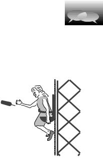
B. Sally is on an amusement park ride which begins with her chair being |
|
hoisted straight up a tower at a constant speed of 60 miles/hour. Despite stern |
|
warnings from her father that he’ll take her home the next time she |
|
misbehaves, she decides that as a scientific experiment she really needs to |
|
release her corndog over the side as she’s on the way up. She does not throw |
|
it. She simply sticks it out of the car, lets it go, and watches it against the |
|
background of the sky, with no trees or buildings as reference points. What |
|
does the corndog’s motion look like as observed by Sally? Does its speed ever |
|
appear to her to be zero? What acceleration does she observe it to have: is it |
|
ever positive? negative? zero? What would her enraged father answer if asked |
|
for a similar description of its motion as it appears to him, standing on the |
|
ground? |
|
C. Can an object maintain a constant acceleration, but meanwhile reverse the |
|
direction of its velocity? |
|
D. Can an object have a velocity that is positive and increasing at the same |
|
time that its acceleration is decreasing? |
|
E. The four figures show a refugee from a Picasso painting blowing on a rolling |
|
water bottle. In some cases the person’s blowing is speeding the bottle up, but |
Discussion question B. |
in others it is slowing it down. The arrow inside the bottle shows which |
|
Section 3.3 Positive and Negative Acceleration |
83 |
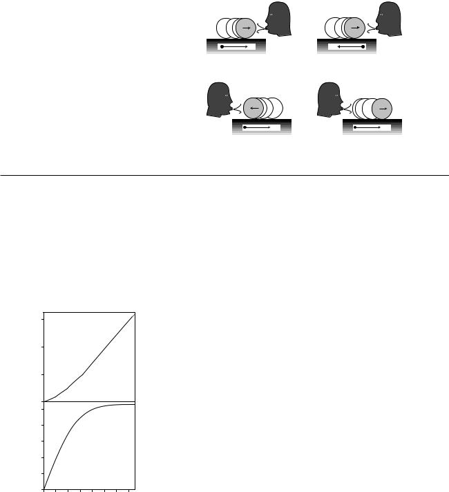
direction it is going, and a coordinate system is shown at the bottom of each figure. In each case, figure out the plus or minus signs of the velocity and acceleration. It may be helpful to draw a v-t graph in each case.
(a) |
(b) |
x |
x |
(c) |
(d) |
x |
x |
3.4 Varying Acceleration
x (m)
v (m/s)
600
400
200
0
50
40
30
20
10
0
0 |
2 |
4 |
6 |
8 |
10 12 14 |
|
|
|
t (s) |
|
|
So far we have only been discussing examples of motion for which the v-t graph is linear. If we wish to generalize our definition to v-t graphs that are more complex curves, the best way to proceed is similar to how we defined velocity for curved x-t graphs:
definition of acceleration
The acceleration of an object at any instant is the slope of the tangent line passing through its v-versus-t graph at the relevant point.
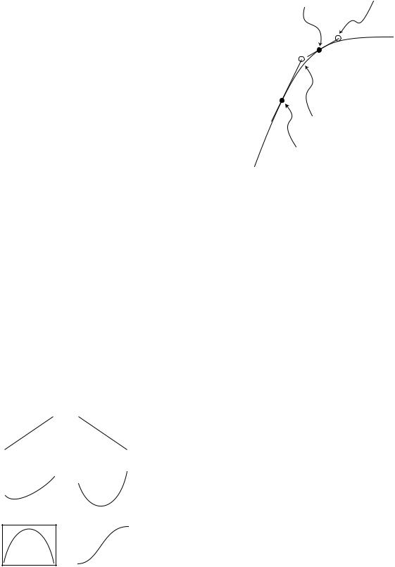
Example: a skydiver
Question: The graphs show the results of a fairly realistic computer simulation of the motion of a skydiver, including the effects of air friction. The x axis has been chosen pointing down, so x is increasing as she falls. Find (a) the skydiver’s acceleration at t=3.0 s, and also (b) at t=7.0 s.
Solution: I’ve added tangent lines at the two points in question.
(a) To find the slope of the tangent line, I pick two points on the
84 |
Chapter 3 Acceleration and Free Fall |
x |
a=0 |
x |
a=0 |
|
|
||||
|
|
|||
|
|
|
|
|
|
t |
|
t |
|
|
|
|
|
|
|
small, |
|
large, |
|
x |
positive |
x |
positive |
|
|
a |
|
a |
|
|
|
|
|
|
|
t |
|
t |
|
|
|
|
|
|
x |
large, |
x |
a<0 |
|
|
||||
negative |
a>0 |
|||
|
|
|||
|
a |
|
|
|
|
t |
|
t |
|
|
|
(7.0 s, 47 m/s) |
|
(9.0 s, 52 m/s) |
|||||||||
|
|
|
|
|
|
|
|
|
|
|||||
|
50 |
|
|
|
|
|
|
|
|
|
|
|
|
|
|
|
|
|
|
|
|
|
|
|
|
|
|
|
|
|
|
|
|
|
|
|
|
|
|
|
|
|
|
|
|
40 |
|
|
|
|
|
|
|
|
|
|
|
|
|
|
|
|
|
|
|
|
|
|
|
|
|
|
|
|
v (m/s) |
30 |
|
|
|
|
|
|
|
|
|
|
|
|
|
|
|
|
|
|
|
|
|
|
|
|
|
|
||
20 |
|
|
|
|
(5.0 s, 42 m/s) |
|
|
|
||||||
|
|
|
|
|
|
|
|
|||||||
|
|
|
|
|
|
|
|
|
||||||
|
10 |
|
|
|
(3.0 s, 28 m/s) |
|
|
|
|
|
||||
|
|
|
|
|
|
|
|
|
||||||
|
|
|
|
|
|
|
|
|
|
|||||
|
0 |
|
|
|
|
|
|
|
|
|
|
|
|
|
|
|
|
|
|
|
|
|
|
|
|
|
|
|
|
|
0 |
2 |
4 |
6 |
8 |
10 |
12 |
14 |
|
|||||
|
|
|
|
|
|
t (s) |
|
|
|
|
|
|
|
|
line (not necessarily on the actual curve): (3.0 s, 28 m/s) and (5.0
s, 42 m/s). The slope of the tangent line is (42 m/s-28 m/s)/(5.0 s - 3.0 s)=7.0 m/s2.
(b) Two points on this tangent line are (7.0 s, 47 m/s) and (9.0 s, 52 m/s). The slope of the tangent line is (52 m/s-47 m/s)/(9.0 s - 7.0 s)=2.5 m/s2.
Physically, what’s happening is that at t=3.0 s, the skydiver is not yet going very fast, so air friction is not yet very strong. She therefore has an acceleration almost as great as g. At t=7.0 s, she is moving almost twice as fast (about 100 miles per hour), and air friction is extremely strong, resulting in a significant departure from the idealized case of no air friction.
In the above example, the x-t graph was not even used in the solution of the problem, since the definition of acceleration refers to the slope of the v-t graph. It is possible, however, to interpret an x-t graph to find out something about the acceleration. An object with zero acceleration, i.e. constant velocity, has an x-t graph that is a straight line. A straight line has no curvature. A change in velocity requires a change in the slope of the x-t graph, which means that it is a curve rather than a line. Thus acceleration relates to the curvature of the x-t graph. Figure (c) shows some examples.
In the skydiver example, the x-t graph was more strongly curved at the beginning, and became nearly straight at the end. If the x-t graph is nearly straight, then its slope, the velocity, is nearly constant, and the acceleration is therefore small. We can thus interpret the acceleration as representing the curvature of the x-t graph. If the “cup” of the curve points up, the acceleration is positive, and if it points down, the acceleration is negative.
Since the relationship between a and v is analogous to the relationship
Section 3.3 Positive and Negative Acceleration |
85 |
a (m/s2) v (m/s) x (m)
10 |
|
|
|
|
|
|
|
|
|
|
|
|
|
|
|
|
|
(m)x |
600 |
|
|
|
|
|
|
|
|
|
|
|
|
|
|
|
|
|
|
|
|
|
|
|
|
|
|
|
|
|
|
|
|
|
|
|
|
|
|
|
|
|
|
|
|
|
|
|
|
|
|
|
|
|
|
|
|
|
|
|
|
||||
|
|
|
|
|
|
|
|
|
|
|
|
|
|
|
|
|
400 |
|
|
|
|
|
|
|
|
|
|
|
|
|
|
|
|
|
|
position |
|||||
5 |
|
|
|
|
|
|
|
|
|
|
|
|
|
|
|
|
|
|
|
|
|
|
|
|
|
|
|
|
|
|
|
|
|
|
|
|
|||||
|
|
|
|
|
|
|
|
|
|
|
|
|
|
|
|
|
|
|
|
|
|
|
|
|
|
|
|
|
|
|
|
|
|
|
|
|
|||||
|
|
|
|
|
|
|
|
|
|
|
|
|
|
|
|
|
|
|
200 |
|
|
|
|
|
|
|
|
|
|
|
|
|
|
|
|
|
|
||||
|
|
|
|
|
|
|
|
|
|
|
|
|
|
|
|
|
|
|
|
|
|
|
|
|
|
|
|
|
|
|
|
|
|
|
|
||||||
0 |
|
|
|
|
|
|
|
|
|
|
|
|
|
|
|
|
|
|
|
|
|
|
|
|
|
|
|
|
|
|
|
|
|
|
|
|
|
||||
|
|
|
|
|
|
|
|
|
|
|
|
|
|
|
|
|
|
|
|
|
|
|
|
|
|
|
|
|
|
|
|
|
|
|
|
|
|||||
|
|
|
|
|
|
|
|
|
|
|
|
|
|
|
|
|
|
|
0 |
|
|
|
|
|
|
|
|
|
|
|
|
|
|
|
|
|
|
|
|||
|
|
|
|
|
|
|
|
|
|
|
|
|
|
|
|
|
|
|
|
|
|
|
|
|
|
|
|
|
|
|
|
|
|
|
|
|
slope of |
|
|
||
|
|
|
|
|
|
|
|
|
|
|
|
|
|
|
|
|
|
|
|
|
|
|
|
|
|
|
|
|
|
|
|
|
|
|
|
|
|
|
|||
4 |
|
|
|
|
|
|
|
|
|
|
|
|
|
|
|
|
|
|
(m/s) |
50 |
|
|
|
|
|
|
|
|
|
|
|
|
|
|
|
|
|
tangent line |
|
|
|
|
|
|
|
|
|
|
|
|
|
|
|
|
|
|
|
|
|
|
|
|
|
|
|
|
|
|
|
|
|
|
|
|
|
|
|
|
|||||
|
|
|
|
|
|
|
|
|
|
|
|
|
|
|
|
|
|
40 |
|
|
|
|
|
|
|
|
|
|
|
|
|
|
|
|
|
|
|
|
|
||
|
|
|
|
|
|
|
|
|
|
|
|
|
|
|
|
|
|
|
|
|
|
|
|
|
|
|
|
|
|
|
|
|
|
velocity curvature |
|||||||
|
|
|
|
|
|
|
|
|
|
|
|
|
|
|
|
|
|
|
|
|
|
|
|
|
|
|
|
|
|
|
|
|
|
|
|
||||||
3 |
|
|
|
|
|
|
|
|
|
|
|
|
|
|
|
|
|
|
30 |
|
|
|
|
|
|
|
|
|
|
|
|
|
|
|
|
|
|
||||
|
|
|
|
|
|
|
|
|
|
|
|
|
|
|
|
|
|
|
|
|
|
|
|
|
|
|
|
|
|
|
|
|
|
|
|
||||||
2 |
|
|
|
|
|
|
|
|
|
|
|
|
|
|
|
|
|
|
v |
20 |
|
|
|
|
|
|
|
|
|
|
|
|
|
|
|
|
|
|
|||
|
|
|
|
|
|
|
|
|
|
|
|
|
|
|
|
|
|
|
|
|
|
|
|
|
|
|
|
|
|
|
|
|
|
|
|
|
=rate of change of position |
||||
1 |
|
|
|
|
|
|
|
|
|
|
|
|
|
|
|
|
|
|
|
10 |
|
|
|
|
|
|
|
|
|
|
|
|
|
|
|
|
|
|
|||
|
|
|
|
|
|
|
|
|
|
|
|
|
|
|
|
|
|
|
|
|
|
|
|
|
|
|
|
|
|
|
|
|
|
|
|
|
|
|
|
||
0 |
|
|
|
|
|
|
|
|
|
|
|
|
|
|
|
|
|
|
|
0 |
|
|
|
|
|
|
|
|
|
|
|
|
|
|
|
|
|
|
slope of |
|
|
|
|
|
|
|
|
|
|
|
|
|
|
|
|
|
|
|
|
|
|
|
|
|
|
|
|
|
|
|
|
|
|
|
|
|
|
|
|
|
|||
|
|
|
|
|
|
|
|
|
|
|
|
|
|
|
|
|
) |
|
|
|
|
|
|
|
|
|
|
|
|
|
|
|
|
|
|
|
tangent line |
|
|
||
|
|
|
|
|
|
|
|
|
|
|
|
|
|
|
|
|
2 |
|
|
|
|
|
|
|
|
|
|
|
|
|
|
|
|
|
|
|
|
|
|
||
1 |
|
|
|
|
|
|
|
|
|
|
|
|
|
|
|
|
|
|
a (m/s |
5 |
|
|
|
|
|
|
|
|
|
|
|
|
|
|
|
|
|
|
acceleration |
||
|
|
|
|
|
|
|
|
|
|
|
|
|
|
|
|
|
|
|
|
|
|
|
|
|
|
|
|
|
|
|
|
|
|
|
|
||||||
|
|
|
|
|
|
|
|
|
|
|
|
|
|
|
|
|
|
|
|
|
|
|
|
|
|
|
|
|
|
|
|
|
|
|
|
|
|||||
|
|
|
|
|
|
|
|
|
|
|
|
|
|
|
|
|
|
|
|
|
|
|
|
|
|
|
|
|
|
|
|
|
|
|
|
|
|||||
|
|
|
|
|
|
|
|
|
|
|
|
|
|
|
|
|
|
|
|
|
|
|
|
|
|
|
|
|
|
|
|
|
|
|
|
|
|
||||
|
|
|
|
|
|
|
|
|
|
|
|
|
|
|
|
|
|
|
|
|
|
|
|
|
|
|
|
|
|
|
|
|
|
|
|
|
|
|
=rate of change of velocity |
||
0 |
|
|
|
|
|
|
|
|
|
|
|
|
|
|
|
|
|
|
|
0 |
|
|
|
|
|
|
|
|
|
|
|
|
|
|
|
|
|
|
|
|
|
0 |
1 |
2 |
3 |
4 |
5 |
|
|
0 2 4 6 8 101214 |
|
|
|
||||||||||||||||||||||||||||||
|
|
|
|
|
|
|
t (s) |
|
|
|
|
|
|
|
|
|
|
|
|
|
|
t (s) |
(c) |
||||||||||||||||||
|
|
|
|
(a) |
|
|
|
|
|
|
|
|
|
|
|
|
|
|
|
|
(b) |
||||||||||||||||||||
|
|
|
|
|
|
|
|
|
|
|
|
|
|
|
|
|
|
|
|
|
|
|
|||||||||||||||||||
between v and x, we can also make graphs of acceleration as a function of time, as shown in figures (a) and (b) above.
Figure (c) summarizes the relationships among the three types of graphs.
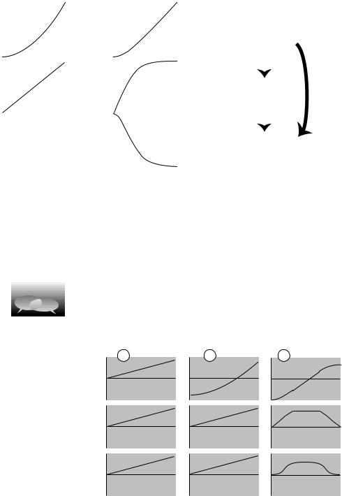
Discussion questions
A. Describe in words how the changes in the a-t graph for the skydiver relate
to the behavior of the v-t graph.
B. Explain how each set of graphs contains inconsistencies.
1 |
2 |
3 |
x |
x |
x |
v |
v |
v |
|
|
|
a |
a |
a |
|
|
|
t |
t |
t |
Discussion question B. |
|
|
86 |
Chapter 3 Acceleration and Free Fall |
3.5The Area Under the Velocity-Time Graph
|
20 |
(a) |
|
|
|
(m/s) |
10 |
|
|
|
|
v |
|
|
|
|
|
|
|
|
|
|
|
|
0 |
|
|
|
|
|
0 |
2 |
4 |
6 |
8 |
|
|
|
t (s) |
|
|
A natural question to ask about falling objects is how fast they fall, but Galileo showed that the question has no answer. The physical law that he discovered connects a cause (the attraction of the planet Earth’s mass) to an effect, but the effect is predicted in terms of an acceleration rather than a velocity. In fact, no physical law predicts a definite velocity as a result of a specific phenomenon, because velocity cannot be measured in absolute terms, and only changes in velocity relate directly to physical phenomena.
The unfortunate thing about this situation is that the definitions of velocity and acceleration are stated in terms of the tangent-line technique, which lets you go from x to v to a, but not the other way around. Without a technique to go backwards from a to v to x, we cannot say anything quantitative, for instance, about the x-t graph of a falling object. Such a technique does exist, and I used it to make the x-t graphs in all the examples above.
|
20 |
(b) |
|
|
|
|
|
|
|
|
|
(m/s) |
10 |
|
|
|
|
v |
|
|
|
|
|
|
|
|
|
|
|
|
0 |
|
|
|
|
|
0 |
2 |
4 |
6 |
8 |
|
|
|
t (s) |
|
|
|
20 |
(c) |
|
|
|
v (m/s) |
10 |
|
|
|
|
|
|
|
|
|
|
|
0 |
|
|
|
|
|
0 |
2 |
4 |
6 |
8 |
|
|
|
t (s) |
|
|
20 (d)
(m/s)v |
10 |
|
|
|
0 |
0 |
2 |
4 |
6 |
8 |
t (s)
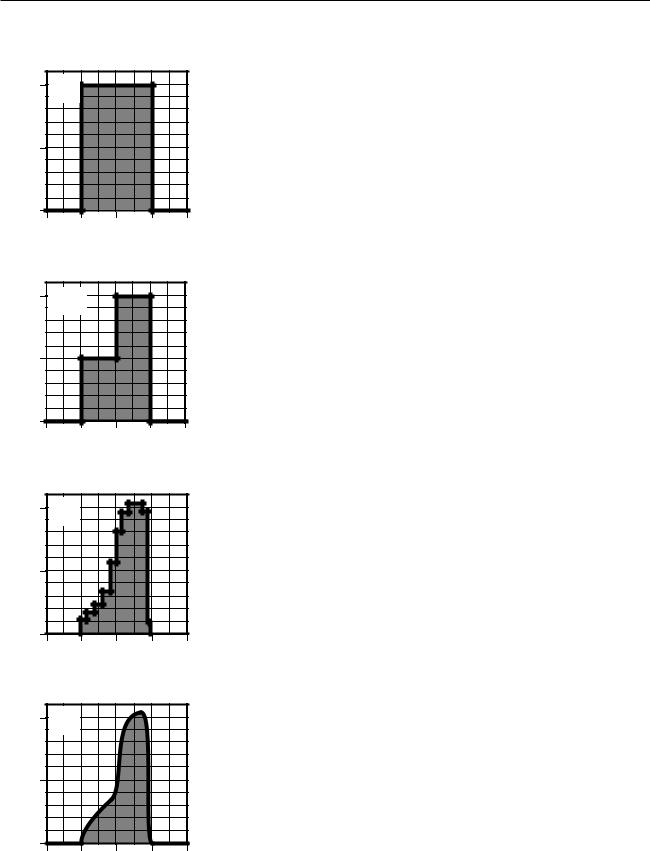
First let’s concentrate on how to get x information out of a v-t graph. In example (a), an object moves at a speed of 20 m/s for a period of 4.0 s. The distance covered is x=v t=(20 m/s)x(4.0 s)=80 m. Notice that the quantities being multiplied are the width and the height of the shaded rectangle
— or, strictly speaking, the time represented by its width and the velocity represented by its height. The distance of x=80 m thus corresponds to the area of the shaded part of the graph.
The next step in sophistication is an example like (b), where the object moves at a constant speed of 10 m/s for two seconds, then for two seconds at a different constant speed of 20 m/s. The shaded region can be split into a small rectangle on the left, with an area representing x=20 m, and a taller one on the right, corresponding to another 40 m of motion. The total distance is thus 60 m, which corresponds to the total area under the graph.
An example like (c) is now just a trivial generalization; there is simply a large number of skinny rectangular areas to add up. But notice that graph
(c) is quite a good approximation to the smooth curve (d). Even though we have no formula for the area of a funny shape like (d), we can approximate its area by dividing it up into smaller areas like rectangles, whose area is easier to calculate. If someone hands you a graph like (d) and asks you to find the area under it, the simplest approach is just to count up the little rectangles on the underlying graph paper, making rough estimates of fractional rectangles as you go along.
Section 3.5 The Area Under the Velocity-Time Graph |
87 |
20
10
v (m/s)
0
0
|
|
|
0.5 m |
|
|
1 m |
1.5 m |
|
|
1 m |
1.5 m |
|
|
1.5 m |
1.5 m |
|
|
2 m |
1.5 m |
|
|
2 m |
1.5 m |
|
|
2 m |
1.5 m |
|
0.5 m |
2 m |
1.5 m |
|
2 m |
2 m |
1.5 m |
1 m |
2 m |
2 m |
1.5 m |
2 m |
2 m |
2 m |
1.5 m |
|
|
|
|
2 |
4 |
6 |
8 |
|
t (s) |
|
|
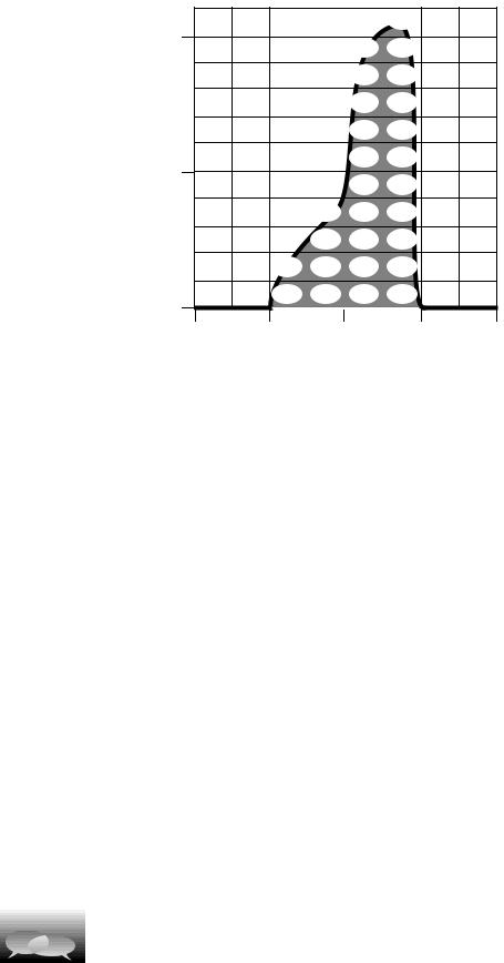
That’s what I’ve done above. Each rectangle on the graph paper is 1.0 s wide and 2 m/s tall, so it represents 2 m. Adding up all the numbers gives
x=41 m. If you needed better accuracy, you could use graph paper with smaller rectangles.
It’s important to realize that this technique gives you x, not x. The v-t graph has no information about where the object was when it started.
The following are important points to keep in mind when applying this technique:
•If the range of v values on your graph does not extend down to zero, then you will get the wrong answer unless you compensate by adding in the area that is not shown.
•As in the example, one rectangle on the graph paper does not necessarily correspond to one meter of distance.
•Negative velocity values represent motion in the opposite direction, so area under the t axis should be subtracted, i.e. counted as “negative area.”
•Since the result is a x value, it only tells you xafter-xbefore, which may be less than the actual distance traveled. For instance, the object could come back to its original position at the end, which would correspond to x=0, even though it had actually moved a nonzero distance.
Finally, note that one can find v from an a-t graph using an entirely analogous method. Each rectangle on the a-t graph represents a certain amount of velocity change.
Discussion question
Roughly what would a pendulum’s v-t graph look like? What would happen when you applied the area-under-the-curve technique to find the pendulum’s
x for a time period covering many swings?
88 |
Chapter 3 Acceleration and Free Fall |
3.6Algebraic Results for Constant Acceleration
v |
t |
v |
vo |
t |
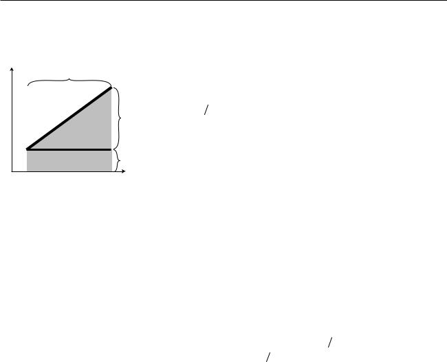
Although the area-under-the-curve technique can be applied to any graph, no matter how complicated, it may be laborious to carry out, and if fractions of rectangles must be estimated the result will only be approximate. In the special case of motion with constant acceleration, it is possible to find a convenient shortcut which produces exact results. When the acceleration is constant, the v-t graph is a straight line, as shown in the figure. The area under the curve can be divided into a triangle plus a rectangle, both of whose areas can be calculated exactly: A=bh for a rect-
angle and A=1 2 bh for a triangle. The height of the rectangle is the initial velocity, vo, and the height of the triangle is the change in velocity from
beginning to end, |
v. The object’s x is therefore given by the equation |
||
Dx = v Dt + 1 v |
t |
. This can be simplified a little by using the definition of |
|
o |
2 |
|
|
acceleration, a= |
v/ |
t to eliminate v, giving |
|
[motion with constant acceleration] .
Since this is a second-order polynomial in t, the graph of x versus t is a parabola, and the same is true of a graph of x versus t — the two graphs differ only by shifting along the two axes. Although I have derived the equation using a figure that shows a positive vo, positive a, and so on, it still turns out to be true regardless of what plus and minus signs are involved.
Another useful equation can be derived if one wants to relate the change in velocity to the distance traveled. This is useful, for instance, for finding the distance needed by a car to come to a stop. For simplicity, we start by deriving the equation for the special case of vo=0, in which the final velocity vf is a synonym for v. Since velocity and distance are the variables of interest, not time, we take the equation x = 1 2 a t2 and use t= v/a to
eliminate t. This gives x = 1 2 ( v)2/a, which can be rewritten as
v 2f = 2aDx [motion with constant acceleration, v o = 0] .
For the more general case where v o ¹ 0 , we skip the tedious algebra leading to the more general equation,
v 2f = v 2o+2aDx [motion with constant acceleration] .
To help get this all organized in your head, first let’s categorize the variables as follows:
Variables that change during motion with constant acceleration: x, v, t
Variable that doesn’t change: a
Section 3.6 Algebraic Results for Constant Acceleration |
89 |

If you know one of the changing variables and want to find another, there is always an equation that relates those two:
|
|
vf2 = vo2 + 2a x |
v |
x |
|
||
|
|
a= |
v |
x = v |
o |
t + 1 a t2 |
t |
|
2 |
|
|
t
The symmetry among the three variables is imperfect only because the equation relating x and t includes the initial velocity.
There are two main difficulties encountered by students in applying these equations:
•The equations apply only to motion with constant acceleration. You can’t apply them if the acceleration is changing.
•Students are often unsure of which equation to use, or may cause themselves unnecessary work by taking the longer path around the triangle in the chart above. Organize your thoughts by listing the variables you are given, the ones you want to find, and the ones you aren’t given and don’t care about.
Example
Question: You are trying to pull an old lady out of the way of an oncoming truck. You are able to give her an acceleration of 20 m/ s2. Starting from rest, how much time is required in order to move her 2 m?
Solution: First we organize our thoughts:
Variables given: |
x, a, vo |
Variables desired: |
t |
Irrelevant variables: |
vf |
Consulting the triangular chart above, the equation we need is clearly x = vo t + 12a t 2 , since it has the four variables of interest and omits the irrelevant one. Eliminating the vo term and
solving for t gives t = |
2 x |
=0.4 s. |
|
a |
|
Discussion questions
A Check that the units make sense in the three equations derived in this
section.
B. In chapter 1, I gave examples of correct and incorrect reasoning about proportionality, using questions about the scaling of area and volume. Try to translate the incorrect modes of reasoning shown there into mistakes about the following question: If the acceleration of gravity on Mars is 1/3 that on Earth, how many times longer does it take for a rock to drop the same distance on Mars?
90 |
Chapter 3 Acceleration and Free Fall |