

Chapter 7- Properties of Convolution |
133 |
Associative Property
Is it possible to convolve three or more signals? The answer is yes, and the associative property describes how: convolve two of the signals to produce an intermediate signal, then convolve the intermediate signal with the third signal. The associative property provides that the order of the convolutions doesn't matter. As an equation:
EQUATION 7-7
The associative property of convolution describes how three or more signals are convolved.
( a [n ] ( b [n ] ) ( c [n ] ' a [n ] ( ( b [n ] ( c [n ] )
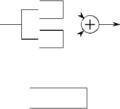
The associative property is used in system theory to describe how cascaded systems behave. As shown in Fig. 7-9, two or more systems are said to be in a cascade if the output of one system is used as the input for the next system. From the associative property, the order of the systems can be rearranged without changing the overall response of the cascade. Further, any number of cascaded systems can be replaced with a single system. The impulse response of the replacement system is found by convolving the impulse responses of all of the original systems.
IF
x[n]  h1[n]
h1[n] 
 h2[n]
h2[n]  y[n]
y[n]
THEN
x[n] 
 h2[n]
h2[n] 
 h1[n]
h1[n]  y[n]
y[n]
ALSO
x[n] 
 h1[n]
h1[n]  h2[n]
h2[n]  y[n]
y[n]
FIGURE 7-9
The associative property in system theory. The associative property provides two important characteristics of cascaded linear systems. First, the order of the systems can be rearranged without changing the overall operation of the cascade. Second, two or more systems in a cascade can be replaced by a single system. The impulse response of the replacement system is found by convolving the impulse responses of the stages being replaced.
134 |
The Scientist and Engineer's Guide to Digital Signal Processing |
Distributive Property
In equation form, the distributive property is written:
EQUATION 7-8
The distributive property of convolution describes how parallel systems are analyzed.
a [n ]( b [n ] % a [n ]( c [n ] ' a [n ] ( ( b [n ] % c [n ] )
The distributive property describes the operation of parallel systems with added outputs. As shown in Fig. 7-10, two or more systems can share the same input, x[n] , and have their outputs added to produce y[n] . The distributive property allows this combination of systems to be replaced with a single system, having an impulse response equal to the sum of the impulse responses of the original systems.
IF
 h1[n]
h1[n] 
x[n] |
y[n] |
 h2[n]
h2[n] 
THEN
x[n] 
 h1[n] + h2[n]
  y[n]
y[n]
FIGURE 7-10
The distributive property in system theory. The distributive property shows that parallel systems with added outputs can be replaced with a single system. The impulse response of the replacement system is equal to the sum of the impulse responses of all the original systems.
Transference between the Input and Output
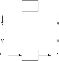
Rather than being a formal mathematical property, this is a way of thinking about a common situation in signal processing. As illustrated in Fig. 7-11, imagine a linear system receiving an input signal, x[n] , and generating an output signal, y[n] . Now suppose that the input signal is changed in some linear way, resulting in a new input signal, which we will call x 3[n]. This results in a new output signal, y 3[n]. The question is, how does the change in
Chapter 7- Properties of Convolution |
135 |
the input signal relate to the change in the output signal? The answer is: the output signal is changed in exactly the same linear way that the input signal was changed. For example, if the input signal is amplified by a factor of two, the output signal will also be amplified by a factor of two. If the derivative is taken of the input signal, the derivative will also be taken of the output signal. If the input is filtered in some way, the output will be filtered in an identical manner. This can easily be proven by using the associative property.
IF
x[n]  h[n]
h[n]  y[n]
y[n]
Linear |
|
Same |
||
|
Linear |
|||
Change |
|
|||
|
Change |
|||
|
|
|
||
|
|
|
|
|
|
|
|
|
|
THEN
x [n] |
h[n] |
y [n] |
FIGURE 7-11
Tranference between the input and output. This is a way of thinking about a common situation in signal processing. A linear change made to the input signal results in the same linear change being made to the output signal.
The Central Limit Theorem
The Central Limit Theorem is an important tool in probability theory because it mathematically explains why the Gaussian probability distribution is observed so commonly in nature. For example: the amplitude of thermal noise in electronic circuits follows a Gaussian distribution; the cross-sectional intensity of a laser beam is Gaussian; even the pattern of holes around a dart board bull's eye is Gaussian. In its simplest form, the Central Limit Theorem states that a Gaussian distribution results when the observed variable is the sum of many random processes. Even if the component processes do not have a Gaussian distribution, the sum of them will.
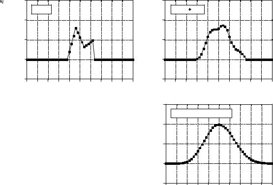
The Central Limit Theorem has an interesting implication for convolution. If a pulse-like signal is convolved with itself many times, a Gaussian is produced. Figure 7-12 shows an example of this. The signal in (a) is an
136 |
The Scientist and Engineer's Guide to Digital Signal Processing |
|
3.00 |
|
|
a. x[n] |
|
Amplitude |
2.00 |
|
1.00 |
||
|
||
|
0.00 |
-1.00 |
|
|
|
-25 -20 -15 -10 -5 |
0 |
5 |
10 15 20 25 |
Sample number
FIGURE 7-12
Example of convolving a pulse waveform with itself. The Central Limit Theorem shows that a Gaussian waveform is produced when an arbitrary shaped pulse is convolved with itself many times. Figure (a) is an example pulse. In (b), the pulse is convolved with itself once, and begins to appear smooth and regular. In (c), the pulse is convolved with itself three times, and closely approximates a Gaussian.
|
18.0 |
|
|
|
|
|
|
|
|
|
|
|
|
b. x[n] |
x[n] |
|
|
|
|
|
|
|
|
Amplitude |
12.0 |
|
|
|
|
|
|
|
|
|
|
6.0 |
|
|
|
|
|
|
|
|
|
|
|
|
|
|
|
|
|
|
|
|
|
|
|
|
0.0 |
|
|
|
|
|
|
|
|
|
|
|
-6.0 |
|
|
|
|
|
|
|
|
|
|
|
-25 |
-20 |
-15 |
-10 |
-5 |
0 |
5 |
10 |
15 |
20 |
25 |
Sample number
1500
c. x[n]  x[n]
x[n]  x[n]
x[n]  x[n]
x[n]
1000
Amplitude |
500 |
|
0 |
-500
-25 -20 -15 -10 -5 |
0 |
5 |
10 15 20 25 |
Sample number
irregular pulse, purposely chosen to be very unlike a Gaussian. Figure (b) shows the result of convolving this signal with itself one time. Figure (c) shows the result of convolving this signal with itself three times. Even with only three convolutions, the waveform looks very much like a Gaussian. In mathematics jargon, the procedure converges to a Gaussian very quickly. The width of the resulting Gaussian (i.e., F in Eq. 2-7 or 2-8) is equal to the width of the original pulse (expressed as F in Eq. 2-7) multiplied by the square root of the number of convolutions.
Correlation
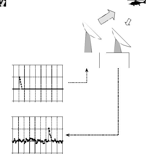
The concept of correlation can best be presented with an example. Figure 7-13 shows the key elements of a radar system. A specially designed antenna transmits a short burst of radio wave energy in a selected direction. If the propagating wave strikes an object, such as the helicopter in this illustration, a small fraction of the energy is reflected back toward a radio receiver located near the transmitter. The transmitted pulse is a specific shape that we have selected, such as the triangle shown in this example. The received signal will consist of two parts: (1) a shifted and scaled version of the transmitted pulse, and (2) random noise, resulting from interfering radio waves, thermal noise in the electronics, etc. Since radio signals travel at a known rate, the speed of
Chapter 7- Properties of Convolution |
137 |
light, the shift between the transmitted and received pulse is a direct measure of the distance to the object being detected. This is the problem: given a signal of some known shape, what is the best way to determine where (or if) the signal occurs in another signal. Correlation is the answer.
Correlation is a mathematical operation that is very similar to convolution. Just as with convolution, correlation uses two signals to produce a third signal. This third signal is called the cross-correlation of the two input signals. If a signal is correlated with itself, the resulting signal is instead called the autocorrelation. The convolution machine was presented in the last chapter to show how convolution is performed. Figure 7-14 is a similar
FIGURE 7-13
Key elements of a radar system. Like other echo location systems, radar transmits a short pulse of energy that is reflected by objects being examined. This makes the received waveform a shifted version of the transmitted waveform, plus random noise. Detection of a known waveform in a noisy signal is the fundamental problem in echo location. The answer to this problem is correlation.
TRANSMIT RECEIVE
|
200 |
|
|
|
|
|
|
|
|
|
amplitude |
100 |
|
|
|
|
|
|
|
|
|
|
|
|
|
|
|
|
|
|
|
|
Transmitted |
0 |
|
|
|
|
|
|
|
|
|
|
|
|
|
|
|
|
|
|
|
|
|
-100 |
|
|
|
|
|
|
|
|
|
|
-10 |
0 |
10 |
20 |
30 |
40 |
50 |
60 |
70 |
80 |
Sample number (or time)
amplitude |
0.2 |
|
0.1 |
||
|
||
Received |
0 |
|
|
-0.1
-10 |
0 |
10 |
20 |
30 |
40 |
50 |
60 |
70 |
80 |
Sample number (or time)
138 |
The Scientist and Engineer's Guide to Digital Signal Processing |
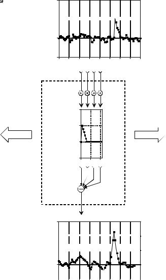
illustration of a correlation machine. The received signal, x[n] , and the cross-correlation signal, y[n] , are fixed on the page. The waveform we are looking for, t[n] , commonly called the target signal, is contained within the correlation machine. Each sample in y[n] is calculated by moving the correlation machine left or right until it points to the sample being worked on. Next, the indicated samples from the received signal fall into the correlation machine, and are multiplied by the corresponding points in the target signal. The sum of these products then moves into the proper sample in the crosscorrelation signal.
The amplitude of each sample in the cross-correlation signal is a measure of how much the received signal resembles the target signal, at that location. This means that a peak will occur in the cross-correlation signal for every target signal that is present in the received signal. In other words, the value of the cross-correlation is maximized when the target signal is aligned with the same features in the received signal.
What if the target signal contains samples with a negative value? Nothing changes. Imagine that the correlation machine is positioned such that the target signal is perfectly aligned with the matching waveform in the received signal. As samples from the received signal fall into the correlation machine, they are multiplied by their matching samples in the target signal. Neglecting noise, a positive sample will be multiplied by itself, resulting in a positive number. Likewise, a negative sample will be multiplied by itself, also resulting in a positive number. Even if the target signal is completely negative, the peak in the cross-correlation will still be positive.
If there is noise on the received signal, there will also be noise on the crosscorrelation signal. It is an unavoidable fact that random noise looks a certain amount like any target signal you can choose. The noise on the cross-correlation signal is simply measuring this similarity. Except for this noise, the peak generated in the cross-correlation signal is symmetrical between its left and right. This is true even if the target signal isn't symmetrical. In addition, the width of the peak is twice the width of the target signal. Remember, the cross-correlation is trying to detect the target signal, not recreate it. There is no reason to expect that the peak will even look like the target signal.
Correlation is the optimal technique for detecting a known waveform in random noise. That is, the peak is higher above the noise using correlation than can be produced by any other linear system. (To be perfectly correct, it is only optimal for random white noise). Using correlation to detect a known waveform is frequently called matched filtering. More on this in Chapter 17.
The correlation machine and convolution machine are identical, except for one small difference. As discussed in the last chapter, the signal inside of the convolution machine is flipped left-for-right. This means that samples numbers: 1, 2, 3 þ run from the right to the left. In the correlation machine this flip doesn't take place, and the samples run in the normal direction.
Chapter 7- Properties of Convolution |
139 |
2
1 


x[n]
0 |
-1
0 |
10 |
20 |
30 |
40 |
50 |
60 |
70 |
80 |
Sample number (or time)
2 |
|
|
1 |
|
|
t[n] |
|
|
0 |
|
|
-1 |
|
|
0 |
10 |
20 |
3
2 


y[n] 1
1 


0 |
-1 |
|
|
|
|
|
|
|
|
|
|
|
|
|
|
|
|
|
|
|
|
|
|
|
0 |
10 |
20 |
30 |
40 |
50 |
60 |
70 |
80 |
|||
|
|
|
Sample number (or time) |
|
|
|
|||||
FIGURE 7-14
The correlation machine. This is a flowchart showing how the cross-correlation of two signals is calculated. In this example, y [n] is the cross-correlation of x [n] and t [n]. The dashed box is moved left or right so that its output points at the sample being calculated in y [n]. The indicated samples from x [n] are multiplied by the corresponding samples in t [n], and the products added. The correlation machine is identical to the convolution machine (Figs. 6-8 and 6-9), except that the signal inside of the dashed box is not reversed. In this illustration, the only samples calculated in y [n] are where t [n] is fully immersed in x [n].
Since this signal reversal is the only difference between the two operations, it is possible to represent correlation using the same mathematics as convolution. This requires preflipping one of the two signals being correlated, so that the left-for-right flip inherent in convolution is canceled. For instance, when a[n]
a n d b[n] , are convolved to produce c[n] , the equation |
is written: |
a [n ]( b [n ] ' c [n ] . In comparison, the cross-correlation of a[n] |
and b[n] can |
140 The Scientist and Engineer's Guide to Digital Signal Processing
be written: a [n ]( b [& n ] ' c [n ] . That is, flipping b [n] left-for-right is accomplished by reversing the sign of the index, i.e., b [& n].
Don't let the mathematical similarity between convolution and correlation fool you; they represent very different DSP procedures. Convolution is the relationship between a system's input signal, output signal, and impulse response. Correlation is a way to detect a known waveform in a noisy background. The similar mathematics is only a convenient coincidence.
Speed
Writing a program to convolve one signal by another is a simple task, only requiring a few lines of code. Executing the program may be more painful. The problem is the large number of additions and multiplications required by the algorithm, resulting in long execution times. As shown by the programs in the last chapter, the time-consuming operation is composed of multiplying two numbers and adding the result to an accumulator. Other parts of the algorithm, such as indexing the arrays, are very quick. The multiply-accumulate is a basic building block in DSP, and we will see it repeated in several other important algorithms. In fact, the speed of DSP computers is often specified by how long it takes to preform a multiply-accumulate operation.
If a signal composed of N samples is convolved with a signal composed of M samples, N × M multiply-accumulations must be preformed. This can be seen from the programs of the last chapter. Personal computers of the mid 1990's requires about one microsecond per multiply-accumulation (100 MHz Pentium using single precision floating point, see Table 4-6). Therefore, convolving a 10,000 sample signal with a 100 sample signal requires about one second. To process a one million point signal with a 3000 point impulse response requires nearly an hour. A decade earlier (80286 at 12 MHz), this calculation would have required three days!
The problem of excessive execution time is commonly handled in one of three ways. First, simply keep the signals as short as possible and use integers instead of floating point. If you only need to run the convolution a few times, this will probably be the best trade-off between execution time and programming effort. Second, use a computer designed for DSP. DSP microprocessors are available with multiply-accumulate times of only a few tens of nanoseconds. This is the route to go if you plan to perform the convolution many times, such as in the design of commercial products.
The third solution is to use a better algorithm for implementing the convolution. Chapter 17 describes a very sophisticated algorithm called FFT convolution. FFT convolution produces exactly the same result as the convolution algorithms presented in the last chapter; however, the execution time is dramatically reduced. For signals with thousands of samples, FFT convolution can be hundreds of times faster. The disadvantage is program complexity. Even if you are familiar with the technique, expect to spend several hours getting the program to run.