Литература / Advanced Digital Signal Processing and Noise Reduction (Saeed V. Vaseghi) / 02 - Noise and distortion

Electrical noise from these sources can be categorized into two basic types: electrostatic and magnetic. These two types of noise are fundamentally different, and thus require different noise-shielding measures. Unfortunately, most of the common noise sources listed above produce combinations of the two noise types, which can complicate the noise reduction problem.

Electrostatic fields are generated by the presence of voltage, with or without current flow. Fluorescent lighting is one of the more common sources of electrostatic noise. Magnetic fields are created either by the flow of electric current or by the presence of permanent magnetism. Motors and transformers are examples of the former, and the Earth's magnetic field is an instance of the latter. In order for noise voltage to be developed in a conductor, magnetic lines of flux must be cut by the conductor. Electric generators function on this basic principle. In the presence of an alternating field, such as that surrounding a 50/60 Hz power line, voltage will be induced into any stationary conductor as the magnetic field expands and collapses. Similarly, a conductor moving through the Earth's magnetic field has a noise voltage generated in it as it cuts the lines of flux.

2.9 Channel Distortions

On propagating through a channel, signals are shaped and distorted by the frequency response and the attenuating characteristics of the channel. There are two main manifestations of channel distortions: magnitude distortion and phase distortion. In addition, in radio communication, we have the

Figure 2.7 Illustration of channel distortion: (a) the input signal spectrum, (b) the channel frequency response, (c) the channel output.

multi-path effect, in which the transmitted signal may take several different routes to the receiver, with the effect that multiple versions of the signal with different delay and attenuation arrive at the receiver. Channel distortions can degrade or even severely disrupt a communication process, and hence channel modelling and equalization are essential components of modern digital communication systems. Channel equalization is particularly important in modern cellular communication systems, since the variations of channel characteristics and propagation attenuation in cellular radio systems are far greater than those of the landline systems. Figure 2.7 illustrates the frequency response of a channel with one invertible and two non-invertible regions. In the non-invertible regions, the signal frequencies are heavily attenuated and lost to the channel noise. In the invertible region, the signal is distorted but recoverable. This example illustrates that the channel inverse filter must be implemented with care in order to avoid undesirable results such as noise amplification at frequencies with a low SNR. Channel equalization is covered in detail in Chapter 15.

2.10 Modelling Noise

The objective of modelling is to characterise the structures and the patterns in a signal or a noise process. To model a noise accurately, we need a structure for modelling both the temporal and the spectral characteristics of the noise. Accurate modelling of noise statistics is the key to high-quality noisy signal classification and enhancement. Even the seemingly simple task of signal/noise classification is crucially dependent on the availability of good signal and noise models, and on the use of these models within a Bayesian framework. Hidden Markov models described in Chapter 5 are good structure for modelling signals or noise.

One of the most useful and indispensable tools for gaining insight into the structure of a noise process is the use of Fourier transform for frequency

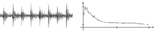
Figure 2.8 Illustration of: (a) the time-waveform of a drill noise, and (b) the frequency spectrum of the drill noise.

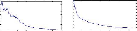
Figure 2.9 Power spectra of car noise in (a) a BMW at 70 mph, and

(b) a Volvo at 70 mph.

analysis. Figure 2.8 illustrates the noise from an electric drill, which, as expected, has a periodic structure. The spectrum of the drilling noise shown in Figure 2.8(a) reveals that most of the noise energy is concentrated in the lower-frequency part of the spectrum. In fact, it is true of most audio signals and noise that they have a predominantly low-frequency spectrum. However, it must be noted that the relatively lower-energy high-frequency part of audio signals plays an important part in conveying sensation and quality. Figures 2.9(a) and (b) show examples of the spectra of car noise recorded from a BMW and a Volvo respectively. The noise in a car is nonstationary, and varied, and may include the following sources:

(a)quasi-periodic noise from the car engine and the revolving mechanical parts of the car;

(b)noise from the surface contact of wheels and the road surface;

(c)noise from the air flow into the car through the air ducts, windows, sunroof, etc;

(d)noise from passing/overtaking vehicles.

The characteristic of car noise varies with the speed, the road surface conditions, the weather, and the environment within the car.

The simplest method for noise modelling, often used in current practice, is to estimate the noise statistics from the signal-inactive periods. In optimal Bayesian signal processing methods, a set of probability models are trained for the signal and the noise processes. The models are then used for the decoding of the underlying states of the signal and noise, and for noisy signal recognition and enhancement.

Bibliography

BELL D.A. (1960) Electrical Noise and Physical Mechanism. Van Nostrand, London.
BENNETT W.R. (1960) Electrical Noise. McGraw-Hill. NewYork. DAVENPORT W.B. and ROOT W.L. (1958) An Introduction to the Theory of
Random Signals and Noise. McGraw-Hill, New York.
GODSILL S.J. (1993) The Restoration of Degraded Audio Signals. Ph.D. Thesis, Cambridge University.
SCHWARTZ M. (1990) Information Transmission, Modulation and Noise. 4th Ed., McGraw-Hill, New York.
EPHRAIM Y. (1992) Statistical Model Based Speech Enhancement Systems. Proc. IEEE 80, 10, pp. 1526–1555.
VAN-TREES H.L. (1971) Detection, Estimation and Modulation Theory. Parts I, II and III. Wiley, New York.