0211109

Having multiplied the both parts of (11.6) (or (11.8)) by ci and summed over i , we

obtain the same result representing the relationship between the Lagrange multipliers:

(n +m)= λ1 +λ2 E

The sample mean energy E (i.e., the sum of the mean potential energy that can be measured in the coordinate space and the mean kinetic energy measured in the momentum space) was used as the estimator of the mean energy in numerical simulations below.

Now, let us turn to the study of statistical fluctuations of a state vector in the problem under consideration. We restrict our consideration to the energy representation in the case when the expansion basis is formed by stationary energy states (that are assumed to be nondegenerate).

Additional condition (11.3) related to the conservation of energy results in the following relationship between the components

δE =∑s−1 (Ejcjδcj +Ejδcjcj )=0. (11.10)

j=0

It turns out that both parts of the equality can be reduced to zero independently if one assumes that a state vector to be estimated involves a time uncertainty, i.e., may differ from the true one by a small time translation. The possibility of such a translation is related to the time-energy uncertainty relation.

The well-known expansion of the psi function in terms of stationary energy states, in view

of time dependence, has the form ( h =1)

ψ(x)= ∑cj exp(−iEj (t −t0 ))ϕj (x)=

j

In the case of estimating the state vector up to translation in time, the transformation c′j = cj exp(iEjt0 )(11.12)

related to arbitrariness of zero-time reference t0 may be used to fit the estimated state vector to the

true one.

The corresponding infinitesimal time translation leads us to the following variation of a state

vector:

δcj =it0Ejcj . (11.13)

Let δc be any variation meeting both the normalization condition and the law of energy conservation. Then, from (10.15) and (11.3) it follows that

∑(δcj )cj =iε1 , (11.14) j

∑(δcj )Ejcj =iε2 , (11.15) j

where ε1 and ε2 are arbitrary small real numbers.

In analogy with Sec. 10, we divide the total variation δc into unavoidable physical fluctuation δ2c and variations caused by the gauge and time invariances:

31

δcj =iαcj +it0Ejcj +δ2cj . (11.16)

We will separate out the physical variation δ2c , so that it fulfills the conditions (11.14)

and (11.15) with a zero right part. It is possible if the transformation parameters α and t0 satisfy the following set of linear equations:

The determinant of (11.17) is the energy variance

σE2 = E2 −E 2 . (11.18)

We assume that the energy variance is a positive number. Then, there exists a unique solution of the set (11.17). If the energy dissipation is equal to zero, the state vector has the only nonzero component. In this case, the gauge transformation and time translation are dependent, since they are reduced to a simple phase shift.

In full analogy with the reasoning on the gauge invariance, one can show that in view of both the gauge invariance and time homogeneity, the transformation satisfying (11.17) provides minimization of the total variance of the variations (sum of squares of the components absolute values). Thus, one may infer that physical fluctuations are minimum possible fluctuations compatible with the conservation of norm and energy.

Assuming that the total variations are reduced to the physical ones, we assume hereafter that

∑(δcj )cj = 0, (11.19) j

∑(δcj )Ejcj = 0. (11.20) j

The relationships found yield (in analogy with Sec. 10) the conditions for the covariance

matrix Σij =δciδcj :

∑(Σijcj )= 0 , (11.21) j

∑(Σij Ejcj )= 0 . (11.22) j

Consider the unitary matrix U + with the following two rows (zero and first):

(U + )0 j = cj , (11.23)

This matrix determines the transition to principle components of the variation

Uij+δcj =δfi . (11.25)

According to (11.19) and (11.20), we have δf0 =δf1 = 0 identically in new variables so

that there remain only s −2 independent degrees of freedom. The inverse transformation is

32

Uδf =δc . (11.26)

On account of the fact that δf0 =δf1 = 0, one may drop two columns (zero and first) in the U matrix turning it into the factor loadings matrix L

i, j = 0,1,...,s −1

It is easily verified that this matrix satisfies the conditions (11.21) and (11.22) resulting from the conservation of norm and energy.

The mean square fluctuation of the psi function is

∫δψδψ dx = ∫δciϕi (x)δcjϕj (x)dx =δciδci =Tr(Σ)= s −2 . (11.33) n +m

The estimation of optimal number of harmonics in the Fourier series, similar to that in Sec. 7, has the form

sopt = r +1 rf (n +m), (11.34)

where the parameters r and f determine the asymptotics for the sum of squares of residuals:

The norm existence implies only that r > 0 . In the case of statistical ensemble of harmonic oscillators with existing energy, r >1. If the energy variance is defined as well, r > 2.

33

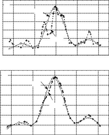
Figure 6 shows how the constraint on energy decreases high-energy noise. The momentumspace density estimator disregarding the constraint on energy (upper plot) is compared to that accounting for the constraint.

Fig. 6 (a) An estimator without the constraint on energy;

(b) An estimator with the constraint on energy.

p

p

The sample of the size of n = m =50 ( n +m =100) was taken from the statistical ensemble of harmonic oscillators. The state vector of the ensemble had three nonzero components ( s =3).

Figure 6 shows the calculation results in bases involving s =3 and functions, respectively. In the latter case, the number of basis functions coincided with the total sample size. Figure 6 shows that in the case when the constraint on energy was taken into account, the 97 additional noise components influenced the result much weaker than in the case without the constraint.

12. Fisher Information and Variational Principle in Quantum Mechanics

The aim of this section is to show a certain relation between the mathematical problem of minimizing the energy by the variational principle in quantum mechanics and the problem of minimizing the Fisher information (more precisely, the Fisher information on the translation parameter) that may be used (and is really used) in some model problems of statistical data analysis (for detail, see [36, 37]).

Let us show that there exists a certain analogy between the Fisher information on the translation parameter and kinetic energy in quantum mechanics. This analogy results in the fact that variational problems of robust statistics are mathematically equivalent to the problems of finding the ground state of a stationary Schrödinger equation [36, 37].

34

Indeed, kinetic energy in quantum mechanics is (see, e.g., [29]; for simplicity, we consider one-dimensional case):

T = − 2hm2 ∫ψ (x)∂2∂ψx(2x)dx = 2hm2 ∫∂∂ψx ∂∂ψx dx . (12.1)

Here, m is the mass of a particle and h is the Planck’s constant.

The last equality follows from integration by parts in view of the fact that the psi function and its derivative are equal to zero at the infinity.

Assume that the psi function is real-valued and equals to the square root of the probability density:

ψ(x)= p(x). (12.2) Then ∂∂ψx = 2 p′p , and hence,

Here, we have taken into account that the Fisher information on the translation parameter, by definition, is [36]

I(p)= +∞∫ p'(x)p 2 p(x) dx . (12.4)

−∞

The Fisher information (12.4) is a functional with respect to the distribution density p(x). Let us consider the following variational problem: it is required to find a distribution density

p(x) minimizing the Fisher information (12.4) at a given constraints on the mean value of the loss

is a potential.

The problem under consideration is linearized if the square root of the density, i.e., psi function is considered instead of the density itself. The variational problem is evidently reduced to minimization of the following functional:

S(ψ )= +∞∫(ψ′(x))2 dx −λ1 (∫ψ 2 (x)dx −1)+

Here, λ1 and λ2 are the Lagrange multipliers providing constraints on the norm of a state vector

and the loss function, respectively.

From the Lagrange-Euler equation it follows the equation for the psi function

−ψ′′+λ2Uψ = λ1ψ . (12.7)

The last equation turns into a stationary Schrödinger equation if one introduces the notation

35

Minimization of kinetic energy at a given constraints on potential energy is equivalent to minimization of the total energy. Therefore, the solution of the corresponding problem is the ground state for a particle in a given field. The corresponding result is well-known in quantum mechanics as the variational principle. It is frequently used to estimate the energy of a ground state.

The kinetic energy representations in two different forms (12.1) and (12.3) are known at least from the works by Bohm on quantum mechanics ([38], see also [30]).

The variational principle considered here is employed in papers on robust statistics developed, among others, by Huber [36]. The aim of robust procedures is, first of all, to find such estimators of distribution parameters (e.g., translation parameters) that would be stable against (weakly sensible to) small deviations of a real distribution from the theoretical one. A basic model in this approach is a certain given distribution (usually, Gaussian distribution) with few given outlying observations.

For example, if the estimator of the translation parameter is of the M- type (i.e., estimators of maximum likelihood type), the maximum estimator variance (due to its efficiency) will be determined by minimal Fisher information characterizing the distribution in a given neighborhood [36].

Minimization of the Fisher information shows the way to construct robust distributions. As is seen from the definition (12.4), the Fisher information is a positive quantity making it possible to estimate the complexity of the density curve. Indeed, the Fisher information is related to the squared derivative of the distribution density; therefore, the more complex, irregular, and oscillating the distribution density, the greater the Fisher information. From this point of view, the simplicity can be achieved by providing minimization of the Fisher information at given constraints. The Fisher information may be considered as a penalty function for the irregularity of the density curve. The introduction of such penalty functions aims at regularization of data analysis problems and is based on the compromise between two tendencies: to obtain the data description as detailed as possible using functions without fast local variations [37, 39-41].

In the work by Good and Gaskins [39], the problem of minimization of smoothing functional, which is equal to the difference between the Fisher information and log likelihood function, is stated in order to approximate the distribution density. The corresponding method is referred to as the maximum penalized likelihood method [40-41].

Among all statistical characteristics, the most popular are certainly the sample mean (estimation of the center of probability distribution) and sample variance (to estimate the deviation). Assuming that these are the only parameters of interest, let us find the simplest distribution (in terms of the Fisher information). The corresponding variational problem is evidently equivalent to the problem of finding the minimum energy solution of the Schrödinger equation (12.7) with a quadratic potential. The corresponding solution (density of the ground state of a harmonic oscillator) is the Gaussian distribution.

If the median and quartiles are used as a given parameters instead of sample mean and variance, which are very sensitive to outlying observations, the family of distributions that are nonparametric analogue of Gaussian distribution and accounting for possible data asymmetry can be found [37].

Conclusions

Let us state a short summary.

The root density estimator is based on the representation of the probability density as a squared absolute value of a certain function, which is referred to as a psi function in analogy with quantum mechanics. The method proposed is an efficient tool to solve the basic problem of statistical data analysis, i.e., estimation of distribution density on the basis of experimental data.

The coefficients of the psi-function expansion in terms of orthonormal set of functions are estimated by the maximum likelihood method providing optimal asymptotic properties of the method (asymptotic unbiasedness, consistency, and asymptotic efficiency). An optimal number of harmonics in the expansion is appropriate to choose, on the basis of the compromise, between two

36

opposite tendencies: the accuracy of the estimation of the function approximated by a finite series increases with increasing number of harmonics, however, the statistical noise level also increases.

The likelihood equation in the root density estimator method has a simple quasilinear structure and admits developing an effective fast-converging iteration procedure even in the case of multiparametric problems. It is shown that an optimal value of the iteration parameter should be found by the maximin strategy. The numerical implementation of the proposed algorithm is considered by the use of the set of Chebyshev-Hermite functions as a basis set of functions.

The introduction of the psi function allows one to represent the Fisher information matrix as well as statistical properties of the sate vector estimator in simple analytical forms. Basic objects of the theory (state vectors, information and covariance matrices etc.) become simple geometrical objects in the Hilbert space that are invariant with respect to unitary (orthogonal) transformations.

A new statistical characteristic, a confidence cone, is introduced instead of a standard confidence interval. The chi-square test is considered to test the hypotheses that the estimated vector equals to the state vector of general population and that both samples are homogeneous.

It is shown that it is convenient to analyze the sample populations (both homogeneous and inhomogeneous) using the density matrix.

The root density estimator may be applied to analyze the results of experiments with micro objects as a natural instrument to solve the inverse problem of quantum mechanics: estimation of psi function by the results of mutually complementing (according to Bohr) experiments. Generalization of the maximum likelihood principle to the case of statistical analysis of mutually complementing experiments is proposed. The principle of complementarity makes it possible to interpret the ill-posedness of the classical inverse problem of probability theory as a consequence of the lacking of the information from canonically conjugate probabilistic space.

The Fisher information matrix and covariance matrix are considered for a quantum statistical ensemble. It is shown that the constraints on the norm and energy are related to the gauge and time translation invariances. The constraint on the energy is shown to result in the suppression of high-frequency noise in a state vector approximated.

The analogy between the variational method in quantum mechanics and certain model problems of mathematical statistics is shown.

References

1.A. N. Tikhonov and V. A. Arsenin. Solutions of ill-posed problems. W.H. Winston. Washington D.C. 1977 .

2.L. Devroye and L. Györfi. Nonparametric Density Estimation: The L1 -View. John Wiley. New York. 1985.

3.V.N. Vapnik and A.R. Stefanyuk. Nonparametric methods for reconstructing probability densities Avtomatika i Telemekhanika 1978. Vol. 39. No. 8. P.38-52.

4.V. N. Vapnik, T. G. Glazkova, V. A. Koscheev et al. Algorithms for dependencies estimations. Nauka. Moscow. 1984 (in Russian).

5.Yu. I. Bogdanov, N. A. Bogdanova, S. I. Zemtsovskii et al. Statistical study of the time-to- failure of the gate dielectric under electrical stress conditions. Microelectronics. 1994. V. 23. N 1. P. 51 – 59. Translated from Mikroelektronika. 1994. V. 23. N1. P. 75-85.

6.Yu. I. Bogdanov, N. A. Bogdanova, S. I. Zemtsovskii Statistical modeling and analysis of data on time dependent breakdown in thin dielectric layers, Radiotekhnika i Electronika. 1995. N.12. P. 1874-1882.

7.M. Rosenblatt Remarks on some nonparametric estimates of a density function // Ann. Math. Statist. 1956. V.27. N3. P.832-837.

37

8.E. Parzen On the estimation of a probability density function and mode // Ann. Math. Statist. 1962. V.33. N3. P.1065-1076.

9.E. A. Nadaraya On Nonparametric Estimators of Probability Density and Regression, Teoriya Veroyatnostei i ee Primeneniya. 1965. V. 10. N. 1. P. 199-203.

10.E. A. Nadaraya Nonparametric Estimation of Probability Densities and Regression Curves. Kluwer Academic Publishers. Boston. 1989.

11.J.S. Marron An asymptotically efficient solution to the bandwidth problem of kernel density estimation. // Ann. Statist. 1985. V.13. №3. P.1011-1023.

12.J.S. Marron A Comparison of cross-validation techniques in density estimation // Ann. Statist. 1987. V.15. №1. P.152-162.

13.B.U. Park, J.S. Marron Comparison of data-driven bandwidth selectors // J. Amer. Statist. Assoc. 1990. V.85. №409. P.66-72.

14.S.J. Sheather, M.C. Jones A reliable data-based bandwidth selection method for kernel density estimation // J. Roy. Statist. Soc. B. 1991. V.53. №3. P.683-690.

15.A. I. Orlov Kernel Density Estimators in Arbitrary Spaces. in: Statistical Methods for Estimation and Testing Hypotheses. P. 68-75. Perm'. 1996 (in Russian).

16.A. I. Orlov Statistics of Nonnumerical Objects. Zavodskaya Laboratoriya. Diagnostika Materialov. 1990. V. 56. N. 3. P. 76-83.

17.N. N. Chentsov (Čensov) Evaluation of unknown distribution density based on observations. Doklady. 1962. V. 3. P.1559 - 1562.

18.N. N. Chentsov (Čensov) Statistical Decision Rules and Optimal Inference. Translations of Mathematical Monographs. American Mathematical Society. Providence. 1982 (Translated from Russian Edition. Nauka. Moscow. 1972).

19.G.S. Watson Density estimation by orthogonal series. Ann. Math. Statist. 1969. V.40. P.14961498.

20.G. Walter Properties of hermite series estimation of probability density. Ann. Statist. 1977. V.5. N6. P.1258-1264.

21.G. Walter, J. Blum Probability density estimation using delta sequences // Ann. Statist. 1979. V.7. №2. P. 328-340.

22.H. Cramer Mathematical Methods of Statistics, Princeton University Press, Princeton, 1946.

23.A. V. Kryanev Application of Modern Methods of Parametric and Nonparametric Statistics in Experimental Data Processing on Computers, MIPhI, Moscow, 1987 (in Russian).

24.R.A. Fisher On an absolute criterion for fitting frequency curves // Massager of Mathematics. 1912. V.41.P.155-160.

25.R.A. Fisher On mathematical foundation of theoretical statistics // Phil. Trans. Roy. Soc. (London). Ser. A. 1922. V.222. P. 309 – 369.

26.M. Kendall and A. Stuart The Advanced Theory of Statistics. Inference and Relationship. U.K. Charles Griffin. London. 1979.

38

27.I. A. Ibragimov and R. Z. Has'minskii Statistical Estimation: Asymptotic Theory. Springer. New York. 1981.

28.S. A. Aivazyan and I. S. Enyukov, and L. D. Meshalkin Applied Statistics: Bases of Modelling and Initial Data Processing. Finansy i Statistika. Moscow. 1983 (in Russian).

29.L. D. Landau and E. M. Lifschitz Quantum Mechanics (Non-Relativistic Theory). 3rd ed. Pergamon Press. Oxford. 1991.

30.D. I. Blokhintsev Principles of Quantum Mechanics, Allyn & Bacon, Boston, 1964.

31.V. V. Balashov and V. K. Dolinov. Quantum mechanics. Moscow University Press. Moscow. 1982 (in Russian).

32.A. N. Tikhonov, A. B. Vasil`eva, A. G. Sveshnikov Differential Equations. Springer-Verlag. Berlin. 1985.

33.N. S. Bakhvalov, N.P. Zhidkov, G. M. Kobel'kov Numerical Methods. Nauka. Moscow. 1987 (in Russian).

34.N. N. Kalitkin Numerical Methods. Nauka. Moscow. 1978 (in Russian).

35.N. Bohr Selected Scientific Papers in Two Volumes. Nauka. Moscow. 1971 (in Russian).

36.P. J. Huber Robust statistics. Wiley. New York. 1981.

37.Yu. I. Bogdanov Fisher Information and a Nonparametric Approximation of the Distribution Density// Industrial Laboratory. Diagnostics of Materials. 1998. V. 64. N 7. P. 472-477. Translated from Zavodskaya Laboratoriya. Diagnostika Materialov. 1998. V. 64. N. 7. P. 54-60.

38.D. Bohm A suggested interpretation of the quantum theory in terms of “hidden” variables. Part I and II // Phys. Rev. 1952. V.85. P.166-179 and 180-193

39.I.J. Good, R.A. Gaskins Nonparametric roughness penalties for probability densities // Biometrica. 1971. V.58. №2. P. 255-277.

40.C. Gu, C. Qiu Smoothing spline density estimation: Theory. // Ann. Statist. 1993. V. 21. №1. P. 217 – 234.

41.P. Green Penalized likelihood // in Encyclopedia of Statistical Sciences. Update V.2. John Wiley. 1998.

About the Author

Yurii Ivanovich Bogdanov

Graduated with honours from the Physics Department of Moscow State University in 1986. Finished his post-graduate work at the same department in 1989. Received his PhD Degree in physics and mathematics in 1990. Scientific interests include statistical methods in fundamental and engineering researches. Author of more than 40 scientific publications (free electron lasers, applied statistics, statistical modeling for semiconductor manufacture). At present he is the head of the Statistical Methods Laboratory (OAO “Angstrem”, Moscow).

e-mail: bogdanov@angstrem.ru

39