

0211109
.pdfFor the difference of distances between the approximate and exact solutions before and after iteration, we have
ρ′ ≤ ερ , where ε =  1−λmin . (4.9)
The distance between the approximate c(r ) and exact c solutions decreases not slower than infinitely decreasing geometric progression [33]
ρ(c(r ), c)≤ εr ρ(c(0), c)≤ |
|
εr |
ρ(c(0), c(1)). (4.10) |
||||
1−ε |
|||||||
|
|
|
|
|
|||
|
The result obtained implies that the number of iterations required for the distance between |
||||||
the approximate and exact solutions to decrease by the factor of exp(k0 ) is |
|||||||
r0 ≈ |
−2k0 |
|
. (4.11) |
|
|
|
|
ln(1−λ |
) |
|
|
|
|||
|
min |
|
|
|
|
|
|
|
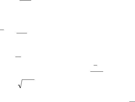
Figure 1 shows an example of the analysis of the iteration procedure convergence. A |
||||||
dependence λmin (α) to |
be found is shown by a solid curve consisted of two segments of |
||||||
parabolas. Besides that, Fig. 1 shows the number of iterations resulted in the same solution for various α at a given accuracy, as well as the approximation of the number of iterations by (4.1) (dotted line). The log likelihood function was controlled in the course of the iteration procedure: the
procedure was stopped when the log likelihood function changed by less than 10−10 .
Fig 1. A dependence of the minimum eigenvalue
of the contracting matrix (left scale) and the number of iterations (right scale) on the iteration parameter
1,0 |
|
|
|
|
5000 |
|
|
|
|
|
|
0,8 |
|
|
Minimum eigenvalue |
1000 |
|
|
|
|
|||
0,6 |
|
|
|
|
500 |
|
Optimum |
|
|
|
|
|
|
|
|
|
|
0,4 |
|
|
|
|
100 |
|
|
|
|
50 |
|
|
|
|
|
|
|
0,2 |
|
|
|
|
|
|
|
|
Number of iterations |
10 |
|
0,0 |
|
|
5 |
||
|
|
|
|
||
|
|
|
|
|
|
|
Stability boundary |
|
|
|
|
-0,2 |
|
|
|
|
1 |
0,0 |
0,2 |
0,4 |
0,6 |
0,8 |
1,0 |
|
|
|
alfa |
|
|
5. Statistical Properties of State Estimator
|
For the sake of simplicity, consider a real valued psi function. |
|||||||||||
|
Let an expansion have the form |
|
|
|
|
|
|
|||||
ψ (x)= |
1 − (c12 +... + cs2−1 )ϕ0 (x)+ c1ϕ1(x)+... + cs −1ϕs −1 (x). |
(5.1) |
|
|||||||||
Here, we have eliminated the coefficient c = |
1−(c2 +...+c2 |
) from the set of parameters to be |
||||||||||
|
|
|
|
|
|
|
|
|
0 |
1 |
s−1 |
|
estimated, since it is expressed via the other coefficients by the normalization condition. |
||||||||||||
|
The parameters |
c1,c2 ,..., cs−1 |
are independent. We will study their asymptotic behavior |
|||||||||
using the Fisher information matrix [22, 26-28] |
|
|
|
|||||||||
Iij (c) |
= n ∫ |
∂ln p(x,c)∂ln p(x,c) |
p(x,c)dx . (5.2) |
|
|
|||||||
∂c |
|
|
∂c |
j |
|
|
|
|
||||
|
|
i |
|
|
|
|
|
|
|
|
|
|
11
It simplifies
Iij = 4n
is of particular importance for our study that the Fisher information matrix drastically
if the psi function is introduced: |
||||
∫ |
∂ψ(x,c)∂ψ(x,c) |
dx . (5.3) |
||
∂c |
∂c |
j |
||
|
i |
|
|
|
|
|
In the case of the expansion (5.1), the information matrix Iij is (s −1)×(s −1) matrix of |
||||||||||||
the form |
|
|
|
|
|
|
|
|
|
1−(c2 |
|
). (5.4) |
||
|
|
|
|
|
|
c c |
j |
|
|
c |
= |
+... +c2 |
||
I |
ij |
= 4n |
δ |
ij |
+ |
i |
|
, |
||||||
c2 |
|
|||||||||||||
|
|
|
|
|
|
|
0 |
|
1 |
s−1 |
|
|||
|
|
|
|
|
|
0 |
|
|
|
|
|
|
|
|
A noticeable feature of the expression (5.4) is its independence on the choice of basis functions. Let us show that only the root density estimator has this property.
Consider the following problem that can be referred to as a generalized orthogonal series density estimator. Let the density p be estimated by a composite function of another (for simplicity, real-valued) function g . The latter function, in its turn, is represented in the form of the expansion in terms of a set of orthonormal functions, i.e.,
s−1
p = p(g), where g(x)= ∑ciϕi (x). (5.5)
i=0
Let the coefficients ci ; i = 0,1,..., s −1 be estimated by the maximum likelihood method.
|
|
|
Consider the following matrix: |
|
|
|
|||||||||
~ |
|
|
|
|
∂ln p(x, c) |
∂ln p(x, c) |
p(x, c)dx = |
|
|
||||||
Iij (c)= n |
∫ |
|
∂ci |
∂c j |
|
|
|
|
|||||||
|
|
|
|
|
|
|
|
|
∂g(x, c)∂g(x, c) . (5.6) |
||||||
|
∫ |
1 ∂p(x, c)∂p(x, c) |
|
∫ |
1 |
∂p 2 |
|||||||||
|
|
|
|
|
|
|
|
|
|
|
|
|
|
||
= n |
|
p |
∂ci |
∂c j |
dx = n |
|
|
|
|
|
∂ci |
∂c j |
dx |
||
|
|
|
|
p |
∂g |
|
|||||||||
The structure of this matrix is simplest if its elements are independent of both the density and basis functions. This can be achieved if (and only if) p(g)satisfies the condition
1 ∂p 2 = const p ∂g
yielding
g = const p . (5.7)
|
Choosing unity as |
the constant in the |
last |
expression, we |
arrive at |
the |
psi function |
||
g =ψ = |
p with the simplest normalization condition (2.3). |
|
|
|
|||||
|
The |
~ |
|
|
|
|
|
|
|
~ |
I |
matrix has the form |
|
|
|
|
|
||
= 4nδij |
i, j = 0,1,...,s −1. (5.8) |
|
|
|
|
|
|||
Iij |
|
|
|
|
|
||||
|
The |
~ |
|
|
|
|
|
|
|
|
I |
matrix under consideration is not the true Fisher information matrix, since the |
|||||||
expansion |
parameters ci |
are dependent. They |
are |
related to each |
other by |
the |
normalization |
||
condition. That is why we will refer to this matrix as a prototype of the Fisher information matrix. As is seen from the asymptotic expansion of the log likelihood function in the vicinity of a
stationary point, statistical properties of the distribution parameters are determined by the quadratic
12

s−1 ~
form ∑Iijδciδcj . Separating out zero component of the variation and taking into account that
i, j =0
|
s−1 |
c c |
|
δc02 |
= ∑ |
i j |
δciδcj (see the expression (5.12) below), we find |
c2 |
|||
|
i, j=1 |
0 |
|
s−1 |
~ |
|
s−1 |
∑Iijδciδc j |
= ∑Iijδciδcj , (5.9) |
||
i, j=0 |
|
|
i, j=1 |
where the true information matrix I has the form of (5.4).
Thus, the representation of the density in the form p =ψ2 (and only this representation)
results in a universal (and simplest) structure of the Fisher information matrix.
In view of the asymptotic efficiency, the covariance matrix of the state estimator is the inverse Fisher information matrix:
Σ(cˆ)= I −1(c) (5.10)
The matrix components are
Σij = 41n (δij −cicj ) i, j =1,..., s −1. (5.11)
Now, let us extend the covariance matrix found by appending the covariance between the c0 component of the state vector and the other components.
Note that |
|
|
|
|
|
|
|
|
|
|
|
|
|
|
|
|
|
|
|
|
|
|
|
|
|
|
|
|||||||
δc |
= |
|
|
∂c0 |
|
δc |
= |
−ci δc |
. (5.12) |
|
|
|
|
|
|
|
|
|||||||||||||||||
|
∂c |
|
|
|
|
|
|
|
|
|
||||||||||||||||||||||||
|
0 |
|
|
|
|
|
|
|
i |
|
|
c |
|
i |
|
|
|
|
|
|
|
|
||||||||||||
|
|
|
|
|
|
i |
|
|
|
|
|
|
|
|
0 |
|
|
|
|
|
|
|
|
|
|
|
|
|
|
|
|
|
||
This yields |
|
|
|
|
|
|
|
−ci |
|
|
|
|
|
|
|
|
|
|
|
|
|
|
|
|
||||||||||
Σ0 j = |
|
|
|
= |
|
|
= |
|
|
|
|
|
|
|
|
|||||||||||||||||||
δc0δc j |
δciδc j |
|
|
|
|
|
|
|
|
|||||||||||||||||||||||||
|
|
|
|
|
|
|
|
|
|
|
||||||||||||||||||||||||
|
|
|
|
|
|
|
|
|
|
|
|
|
|
|
c0 |
|
|
|
−c j ci ) |
|
|
|
|
|
|
|
|
|
|
|||||
= |
|
−Σ ji ci |
|
= |
|
−ci |
(δ ji |
= − |
c0c j |
. (5.13) |
|
|||||||||||||||||||||||
|
|
c0 |
|
|
|
|
|
|
4nc0 |
|
|
|
|
|
4n |
|
|
|
|
|
||||||||||||||
|
|
|
|
|
|
|
|
|
|
|
|
|
|
|
|
|
|
|
|
|
|
|||||||||||||
Similarly, |
|
|
|
|
|
|
cic j |
|
|
|
|
|
|
|
|
|
|
cic j |
|
|
|
|
|
|
|
|||||||||
|
|
|
|
|
|
|
|
|
|
|
|
|
|
|
|
|
|
|
|
|
|
|
|
|
|
|
|
1 |
−c2 |
|
||||
Σ |
|
|
= δc δc |
= |
|
δc δc |
|
= |
Σ |
|
= |
|
||||||||||||||||||||||
00 |
|
|
|
|
j |
|
|
|
ij |
|
0 |
. (5.14) |
||||||||||||||||||||||
|
|
c2 |
|
|
c2 |
|
|
|||||||||||||||||||||||||||
|
0 |
|
0 |
|
|
|
|
|
|
|
|
|
i |
|
|
|
|
|
|
|
|
|
4n |
|
||||||||||
|
|
|
|
|
|
|
|
|
|
|
|
|
|
|
0 |
|
|
|
|
|
|
|
|
|
0 |
|
|
|
|
|
|
|
|
|
Finally, we find that the covariance matrix has the same form as (5.11):
Σ = |
1 |
|
(δ |
ij |
−c c |
) |
i, j |
= |
0,1,...,s |
− |
1. (5.15) |
|
|||||||||||
ij |
4n |
|
i j |
|
|
|
|||||
|
|
|
|
|
|
|
|
|
|
||
This result seems to be almost evident, since the zero component is not singled out from the others (or more precisely, it has been singled out to provide the fulfillment of the normalization condition). From the geometrical standpoint, the covariance matrix (5.15) is a second-order tensor.
Moreover, the covariance matrix (up to a constant factor) is a single second-order tensor satisfying the normalization condition.
Indeed, according to the normalization condition,
δ(cici )= 2ciδci = 0 . (5.16)
Multiplying the last equation by an arbitrary variation δc j and averaging over the statistical ensemble, we find
13
ci E(δciδc j )= Σjici = 0 . (5.17)
Only two different second-order tensors can be constructed on the basis of the vector ci : δij and
cicj . In order to provide the fulfillment of (5.17) following from the normalization condition,
these tensors have to appear in the matrix only in the combination (5.15).
It is useful to consider another derivation of the covariance matrix. According to the normalization condition, the variations δci are dependent, since they are related to each other by
the linear relationship (5.16). In order to make the analysis symmetric (in particular, to avoid expressing one component via the others as it has been done in (5.1)), one may turn to other variables that will be referred to as principle components.
Consider the following unitary (orthogonal) transformation:
Uijδc j = δfi |
i, j = 0,1,..., s −1. (5.18) |
Let the first (to be more precise, zero) row of the transformation matrix coincide with the state vector: U0 j = c j . Then, according to (5.16), the zero variation is identically zero in new
coordinates: δf0 = 0 .
The inverse transformation is
Uij+δf j = δci |
i, j = 0,1,..., s −1 . (5.19) |
|||||||
|
|
In view of the fact that δf0 = 0 |
, the first (more precisely, zero) column of the matrix U + |
|||||
can be eliminated turning the matrix into the factor loadings matrix L . Then |
||||||||
δci |
= Lijδf j |
i = 0,1,..., s −1; |
j =1,..., s −1. (5.20) |
|||||
|
|
The relationship found shows that s components of the state-vector variation are expressed |
||||||
through s −1 principal components (that are independent Gaussian variables). |
||||||||
|
|
In terms of principle components, the Fisher information matrix and covariance matrix are |
||||||
proportional to a unit matrix: |
|
|||||||
Iijf |
= 4nδij |
|
|
i, |
j =1,...,s −1, (5.21) |
|||
Σijf |
= |
|
= |
δij |
i, |
j =1,...,s −1. (5.22) |
||
δfiδf j |
||||||||
4n |
||||||||
|
|
|
|
|
|
|
||
|
|
The |
last relationship particularly shows that the principal variation components are |
|||||
1
independent and have the same variance 4n .
The expression for the covariance matrix of the state vector components can be easily found on the basis of (5.22). Indeed,
Σij =δciδcj = Lik Ljsδfkδfs = Lik Ljs δ4ksn = Lik4Lnjk . (5.23)
In view of the unitarity of the U + matrix, we have
Lik Ljk + cic j = δij . (5.24)
Taking into account two last formulas, we finally find the result presented above:
14

Σ = |
1 |
(δ |
ij |
−c c |
) |
i, j |
= |
0,1,..., s |
− |
1. (5.25) |
|||
|
|
||||||||||||
ij |
|
|
4n |
i j |
|
|
|
||||||
|
|
|
|
|
|
|
|
|
|
|
|||
|
|
|
In quantum mechanics, the matrix |
|
|||||||||
ρij |
=cicj (5.26) |
|
|
|
|
|
|
||||||
is referred to as a density matrix (of a pure state). Thus, |
|||||||||||||
Σ= |
|
1 |
(E −ρ), (5.27) |
|
|
|
|
|
|||||
|
|
|
|
|
|
|
|||||||
|
|
4n |
|
|
|
|
|
|
|
|
|||
where E is the s×s unit matrix. In the diagonal representation,
Σ=UDU+ , (5.28)
where U and D are unitary (orthogonal) and diagonal matrices, respectively.
As is well known from quantum mechanics and readily seen straightforwardly, the density matrix of a pure state has the only (equal to unity) element in the diagonal representation. Thus, in our case, the diagonal of the D matrix has the only element equal to zero (the corresponding
eigenvector is the state vector); whereas the other diagonal elements are equal to 41n (corresponding
eigenvectors and their linear combinations form a subspace that is orthogonal complement to the state vector). The zero element at a principle diagonal indicates that the inverse matrix (namely, the
Fisher information matrix of the s -th order) does not exist. It is clear since there are only s −1 independent parameters in the distribution.
The results on statistical properties of the state vector reconstructed by the maximum likelihood method can be summarized as follows. In contrast to a true state vector, the estimated one involves noise in the form of a random deviation vector located in the space orthogonal to the
true state vector. The components |
|
of the deviation vector (totally, |
s −1 components) |
are |
||||||||||||||||||||||||
asymptotically |
normal |
independent |
|
random variables with the same |
variance |
|
1 |
. In |
the |
|||||||||||||||||||
|
|
|
|
|
|
|
|
|
|
|
|
|
|
|
|
|
|
|
|
|
|
|
|
|
|
4 n |
|
|
aforementioned |
s −1-dimensional space, the deviation vector has an isotropic distribution, and its |
|||||||||||||||||||||||||||
squared length is the random variable |
χs2−1 |
|
, where χs2−1 is the random variable with the chi-square |
|||||||||||||||||||||||||
|
|
|||||||||||||||||||||||||||
|
|
|
|
|
|
|
|
|
|
|
|
|
|
|
|
|
|
4n |
|
|
|
|
|
|
|
|
||
distribution of s −1 degrees of freedom, i.e., |
|
|
|
|
|
|
||||||||||||||||||||||
c |
= (c,c(0)) c(0) +ξ |
i |
|
|
i = 0,1,...,s −1. (5.29) |
|
|
|
|
|
|
|||||||||||||||||
i |
|
|
|
|
|
|
i |
|
|
|
|
|
|
|
|
|
|
|
|
|
|
|
|
|
|
|
||
where |
c(0) |
and |
c are true and estimated state vectors, respectively; (c,c(0))=c c(0) |
, their scalar |
||||||||||||||||||||||||
|
|
|
|
|
|
|
|
|
|
|
|
|
|
|
|
|
|
|
|
|
|
|
|
i i |
|
|
|
|
product; and ξi |
, the deviation vector. The deviation vector is orthogonal to the vector c(0) and has |
|||||||||||||||||||||||||||
|
|
|
|
|
|
|
|
|
|
|
|
|
χ2 |
|
|
|
|
|
|
|
|
|
|
|
|
|
||
the squared length of |
|
|
|
s−1 |
determined by chi-square distribution of s −1 degrees of freedom, i.e., |
|||||||||||||||||||||||
|
|
|
|
|||||||||||||||||||||||||
|
|
|
) |
|
|
|
|
|
|
|
|
|
4n |
|
|
|
|
|
|
|
|
|
|
|
|
|
||
|
|
(0) |
|
|
|
(0) |
|
|
|
|
|
(ξ,ξ)=ξξ |
|
|
|
χs2−1 |
|
|
|
|
|
|
||||||
ξ |
,c |
|
=ξ |
ici |
|
= |
0 |
|
= |
|
|
|
|
|
(5.30) |
|
|
|
|
|
||||||||
|
|
|
|
|
|
|
|
|
|
|
|
|
||||||||||||||||
( |
|
|
|
|
|
|
|
i i |
|
|
|
4n |
|
|
|
|
|
|||||||||||
|
|
|
|
|
|
|
|
|
|
|
|
|
|
|
|
|
|
|
|
|
|
|
|
|
||||
Squaring (5.29), in view of (5.30), we have |
|
|
|
|
|
|
|
|
||||||||||||||||||||
1−(c,c(0))2 = |
χs2−1 |
. (5.31) |
|
|
|
|
|
|
|
|
|
|
|
|
|
|
||||||||||||
4n |
|
|
|
|
|
|
|
|
|
|
|
|
|
|
||||||||||||||
|
|
|
|
|
|
|
|
|
|
|
|
|
|
|
|
|
|
|
|
|
|
|
|
|
|
|
||
15
This expression means that the squared scalar product of the true and estimated state vectors
|
χ2 |
|
is smaller than unity by asymptotically small random variable |
s−1 |
. |
|
||
|
4n |
|
The results found allow one to introduce a new stochastic characteristic, namely, a confidence cone (instead of a standard confidence interval). Let ϑ be the angle between an unknown true state vector c(0) and that c found by solving the likelihood equation. Then,
sin2 ϑ =1−cos2 ϑ =1−(c,c(0))2 = |
χs2−1 |
≤ |
χs2−1,α |
|
. (5.32) |
|
4n |
4n |
|||||
|
|
to the significance level α for the chi-square |
||||
Here, χs2−1,α is the quantile corresponding |
||||||
distribution of s −1 degrees of freedom.
The set of directions determined by the inequality (5.32) constitutes the confidence cone. The axis of a confidence cone is the reconstructed state vector c. The confidence cone covers the
direction of an unknown state vector at a given confidence level P =1−α .
From the standpoint of theory of unitary transformations in quantum mechanics (in our case transformations are reduced to orthogonal), it can be found an expansion basis in (5.1) such that the sum will contain the only nonzero term, namely, the true psi function. This result means that if the best basis is guessed absolutely right and the true state vector is (1,0,0,...,0), the empirical state
vector |
estimated |
by |
the maximum likelihood method will |
be |
the random vector |
|||
(c0 ,c1,c2 ,..., cs−1 ), |
where |
c0 = 1−(c12 +... + cs2−1 ), and |
the |
other components |
||||
|
|
1 |
|
|
|
|
|
|
ci ~ N |
0, |
|
|
i =1,..., s −1 will be independent as it has been noted earlier. |
||||
|
||||||||
|
|
4n |
|
|
|
|
|
|
6. Chi-Square Criterion. Test of the Hypothesis That the Estimated State Vector Equals to the State Vector of a General Population. Estimation of the Statistical Significance of Differences between Two Samples.
Rewrite (5.31) in the form |
|
4n(1−(c,c(0))2 )= χs2−1 . (6.1) |
|
This relationship is a chi-square criterion to test the hypothesis that the state vector |
|
estimated by the maximum likelihood method |
c equals to the state vector of general population |
c(0). |
|
In view of the fact that for n →∞ 1+(c,c(0))→2 , the last inequality may be rewritten in another asymptotically equivalent form
4n∑s−1 (ci |
−ci(0))2 |
= χs2−1 . (6.2) |
i=0 |
|
|
Here, we have taken into account that |
||
∑s−1 (ci −ci(0))2 = ∑s−1 |
(ci 2 −2ci ci(0) +ci(0)2 )= ∑s−1 2(1−ci ci(0)). |
|
i=0 |
i=0 |
i=0 |
As is easily seen, the approach under consideration involves the standard chi-square criterion as a particular case corresponding to a histogram basis. Indeed, the chi-square parameter is usually defined as [22, 28]
16
|
|
s−1 (n − n(0))2 |
|
|
|
|
|
|
|
|
|
|
|||||
χ2 = ∑ |
|
i |
i |
|
, |
|
|
|
|
|
|
|
|
|
|
||
|
|
n(0) |
|
|
|
|
|
|
|
|
|
|
|
||||
|
|
i=0 |
|
i |
|
|
|
|
|
|
|
|
|
|
|
|
|
where ni(0) |
is the number of points expected in i -th interval according to theoretical distribution. |
||||||||||||||||
|
|
In the histogram basis, |
c |
= |
n |
is the empirical state vector and c |
(0) |
= |
ni(0) |
, theoretical |
|||||||
|
|
i |
i |
n |
|||||||||||||
|
|
|
|
|
|
|
|
|
i |
|
n |
|
|
|
|
||
state vector. Then, |
|
|
|
|
|
|
|
|
|
|
|||||||
|
|
|
|
|
|
|
|
|
|
|
|
||||||
χ |
2 |
s−1 |
(c2 −c(0)2 )2 |
|
s |
−1 |
|
(0) |
2 |
|
|
|
|
||||
|
= n∑ |
i |
(0)2 |
|
→ 4n∑(ci −ci |
) . (6.3) |
|
|
|
|
|||||||
|
|
|
|
|
i |
|
|
|
|
|
|
|
|
|
|
||
|
|
i =0 |
|
c i |
|
|
|
i =0 |
|
|
|
|
|
|
|
||
Here, the sign of passage to the limit means that random variables appearing in both sides of (6.3)
have the same distribution. We have used also the asymptotic approximation
ci2 − c(i0 )2 = (ci + ci(0 ))(ci − ci(0 ))→ 2ci(0 )(ci − ci(0 )). (6.4)
Comparing (6.2) and (6.3) shows that the parameter χ2 is a random variable with χ2 -
distribution of s −1 degrees of freedom (if the tested hypothesis is valid). Thus, the standard chisquare criterion is a particular case (corresponding to a histogram basis) of the general approach developed here (that can be used in arbitrary basis).
The chi-square criterion can be applied to test the homogeneity of two different set of observations (samples). In this case, the hypothesis that the observations belong to the same statistical ensemble (the same general population) is tested.
In the case under consideration, the standard chi-square criterion [22, 28] may be represented in new terms as follows:
|
|
|
|
(1) |
|
(2) |
|
2 |
|
|
|
|
|
|
|
|
|
|
|
|
|||
|
|
|
|
ni |
|
− |
ni |
|
|
|
|
|
|
|
|
|
|
|
|
|
|
||
2 |
|
|
|
|
|
|
n1n2 |
|
(1) |
(2) 2 |
|
|
|
|
|
|
|||||||
|
s−1 |
n1 |
|
|
n2 |
|
s−1 |
|
|
|
|
|
|
||||||||||
|
|
|
|
|
|
|
|
|
|
|
|
|
(ci −ci ) |
|
|
|
|
|
|
||||
χ = n1n2 ∑ |
|
|
|
|
|
|
→ 4 |
|
|
∑ |
, (6.5) |
|
|
|
|
|
|||||||
|
|
|
(1) |
(2) |
|
n1 |
|
|
|
|
|
|
|||||||||||
|
|
i=0 |
|
|
ni |
|
+ ni |
|
|
+ n2 i=0 |
|
|
|
|
n(1) |
|
n(2) |
|
|||||
where n |
and |
n |
2 |
|
are the sizes of the first and second samples, respectively; |
and |
, the |
||||||||||||||||
|
1 |
|
|
|
|
|
|
|
|
|
|
|
|
|
|
(1) |
(2) |
|
i |
|
i |
|
|
|
|
|
|
|
|
|
|
|
|
|
|
i -th interval; and |
|
|
|
|
|
||||||
numbers of points in the |
ci |
and ci |
, the empirical state vectors of the |
||||||||||||||||||||
samples. In the left side of (6.5), the chi-square criterion in a histogram basis is presented; in the right side, the same criterion in general case. The parameter χ2 defined in such a way is a
random variable with the χ2 distribution of s −1 degrees of freedom (the sample homogeneity is assumed).
7. Optimization of the Number of Harmonics
Let an exact (usually, unknown) psi function be
ψ(x)= ∑ciϕi (x). (7.1)
i=0∞
Represent the psi-function estimator in the form
s−1
ψˆ (x)= ∑cˆiϕi (x). (7.2)
i=0
Here, the statistical estimators are denoted by caps in order to distinguish them from exact quantities.
17
Comparison of two formulas shows that difference between the exact and estimated psi
functions is caused by two reasons [34]. First, we neglect s -th and higher harmonics by truncating the infinite series. Second, the estimated Fourier series coefficients (with caps) differ from unknown exact values.
Let
cˆi = ci +δci . (7.3)
Then, in view of the basis orthonormality, the squared deviation of the exact function from the approximate one may be written as
s−1 |
∞ |
F(s)= ∫(ψ −ψˆ )2 dx = ∑δci2 +∑ci2 . (7.4) |
|
i=0 |
i=s |
Introduce the notation
∞
Q(s)= ∑ci2 . (7.5)
i=s
By implication, Q(s) is deterministic (not a random) variable. As for the first term, we will consider it as a random variable asymptotically related to the chi-square distribution:
s−1 |
2 |
|
|
∑δci2 ~ |
χs−1 |
, |
|
4n |
|||
i=0 |
|
where χs2−1 is the random variable with the chi-square distribution of s −1 degrees of freedom. Thus, we find that F(s) is a random variable of the form
( )= χ2− + ( )
s 1
F s 4n Q s . (7.6)
We will look for an optimal number of harmonics using the condition for minimum of the function mean value F(s):
F (s)= s4−n1 +Q(s)→ min . (7.7)
Assume that, at sufficiently large s ,
Q(s)= sfr . (7.8)
The optimal value resulting from the condition ∂F∂s(s) = 0 is
sopt = r +1 4rfn . (7.9)
The formula (7.9) has a simple meaning: the Fourier series should be truncated when its coefficients become equal to or smaller than the error, i.e., cs2 ≤ 41n . From (7.8) it follows that
cs2 ≈ |
rf |
. The combination of the last two formulas yields the estimation (7.9). |
|
sr+1 |
|||
|
|
||
|
The coefficients f and r can be calculated by the regression method. The regression |
||
function (7.8) is smoothed by taking a logarithm
18
ln Q(s)= ln f −r ln s . (7.10)
Another way to numerically minimize F (s) is to detect the step when the inequality cs2 ≤ 41n is systematically satisfied. It is necessary to determine that the inequality is met just
systematically in contrast to the case when several coefficients are equal to zero in result of the symmetry of the function.
Our approach to estimate the number of expansion terms does not pretend to high rigor. For instance, strictly speaking, our estimation of the statistical noise level does not directly concern the coefficients in the infinite Fourier series. Indeed, the estimation was performed in the case when the estimated function is exactly described by a finite (preset) number of terms in the Fourier series with coefficients involving certain statistical error due to the finite size of a sample. Moreover, since the function to be determined is unknown (otherwise, there is no a problem), any estimation of the truncation error is approximate, since it is related to the introduction of additional assumptions.
The optimization of the number of terms in the Fourier series may be performed by the Tikhonov regularization methods [1, 34].
8. Numerical Simulations. Chebyshev-Hermite Basis
In this paper, the set of the Chebyshev - Hermite functions corresponding to the stationary states of a quantum harmonic oscillator is used for numerical simulations. In particular, this basis is convenient since the Gaussian distribution in zero-order approximation can be achieved by choosing the ground oscillator state; and adding the contributions of higher harmonics into the state vector provides deviations from the gaussianity.
The set of the Chebyshev-Hermite basis functions is [29, 31]
ϕk (x)= |
|
1 |
|
|
x |
2 |
|
|
|
− |
|
|
|||
|
1/ 2 |
|
|
||||
(2k k! |
Hk (x)exp |
2 |
, k = 0,1,2,.... (8.1) |
||||
|
π ) |
|
|
|
|||
Here, Hk (x) is the Chebyshev-Hermite polynomial of the k -th order. The first two polynomials have the form
H0 (x)=1, (8.2)
H1 (x)= 2x . (8.3)
The other polynomials can be found by the following recurrent relationship:
Hk +1 (x)−2xHk (x)+ 2kHk −1 (x)= 0 . (8.4)
The algorithms proposed here have been tested by the Monte Carlo method using the Chebyshev-Hermite functions for a wide range of distributions (mixture of several Gaussian components, gamma distribution, beta distribution etc.). The results of numerical simulations show that the estimation of the number of terms in the Fourier series is close to optimal. It turns out that the approximation accuracy decays more sharply in the case when less terms than optimal are taken into account than in the opposite case when several extra noise harmonics are allowed for. From the aforesaid, it follows that choosing larger number of terms does not result in sharp deterioration of the approximation results. For example, the approximate density of the mixture of two components weakly varies in the range from 8—10 to 50 and more terms for a sample of several hundreds points.
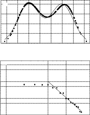
Figure 2 shows an example of comparison of a double-humped curve (dotted line) with an exact distribution (solid line), as well as smoothing the dependence by (7.10) (the sample size is n = 200 ). Note that Figs. 1 and 2 correspond to the same statistical data.
This approach implies that the basis for the psi-function expansion can be arbitrary but it should be preset. In this case, the found results turn out to be universal (independent of basis). This concerns the Fisher information matrix, covariance matrix, chi-square parameter etc. The set of the Chebyshev-Hermite functions can certainly be generalized by introducing translation and scaling
19
parameters that have to be estimated by the maximum likelihood method. The Fisher information matrix, covariance matrix etc. found in such a way would be related only to the Chebyshev-Hermite basis and nothing else.
Fig. 2 (a) An example of comparison of a double-humped curve (dotted line) with an exact distribution (solid line);
(b) smoothing the dependence by (7.10)
P
Q(S)
0,20 |
a) |
0,15
0,10
0,05
0,00
-2 |
-1 |
0 |
1 |
2 |
3 |
4 |
5 |
X
1,000 b) 

0,500
0,100
0,050
0,010
0,005
0,001
1 |
5 |
10 |
S
Practically, the expansion basis can be fixed beforehand if the data describe a well-known physical system (e.g., in atomic systems, the basis is preset by nature in the form of the set of stationary states).
In other cases, the basis has to be chosen in view of the data under consideration. For instance, in the case of the Chebyshev-Hermite functions, it can be easily done if one assumes that the distribution is Gaussian in the zero-order approximation.
Note that the formalism presented here is equally applicable to both one-dimensional and multidimensional data. In the latter case, if the Chebyshev-Hermite functions are used, one may assume that multidimensional normal distribution takes place in the zero-order approximation that, in its turn, can be transformed to the standard form by translation, scale, and rotational transformations.
9. Density Matrix
The density matrix method is a general quantum mechanical method to study inhomogeneous statistical populations (mixtures). The corresponding technique can be used in statistical data analysis as well.
First, for example, consider a case when the analysis of Sec. 6 shows that two statistical samples are inhomogeneous. In this case, the density matrix represented by a mixture of two components can be constructed for the total population:
20