Thermal Analysis of Polymeric Materials

__________________________________________________________________

Description of Sawtooth-modulation Responses

In this Appendix a number of applications of sawtooth modulations are described with modeling and actual results, starting with the sawtooth modulation by utilizing a standard DSC and analysis without Fourier analysis, followed by the analysis of the sawtooth-modulation data after fitting to a Fourier series. Such temperature modulation can be done with any standard DSC which can be programed for a series of consecutive heating and cooling steps.

In the example given, a Perkin-Elmer Pyris-1™ DSC is used with a calibration as described in Sect. 4.3 [1]. The modulation is illustrated in Fig. A.13.1. The heavy line represents the change in sample temperature, the dashed lines represent the

Fig. A.13.1

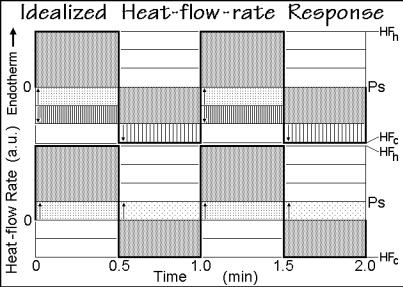
underlying temperature increase by 1.0 K min 1 and the reversing change by ±3 K min 1. Within each cycle, the upper and lower limits of the heat-flow rates, HFh and HFc (proportional to the temperature differences T), are read from the measured temperature-difference response, shown in the lower graph of Fig. A.13.2 for an idealized, instantaneously reacting calorimeter and a sample without latent heat contributions. The response HF(t) is represented by the heavy line, jumping from zero to the heating response in heat-flow rate, HFh, to the cooling response HFc. If the response were not instantaneous, one would have had to wait until the steady states were reached and then extrapolate the steady-state response back to the beginnings of the heating and cooling segments to produce a result similar to the one shown in Fig. A.13.2. For a heat capacity that changes linearly with temperature, the analysis shown next is still possible for the slow response, but a nonlinear change in heat capacity would destroy the stationarity. The reversible heat-flow rate can be

838 Appendix 13–Description of Sawtooth-modulation Response

__________________________________________________________________

Fig. A.13.2

deconvoluted by subtracting <HF(t)> from HF(t) as shown in the lower graph of Fig. A.13.2. During the heating segment, the lightly, vertically dotted area, is part of the positive heat-flow rate HFh. During the cooling segment, the underlying portion of the lightly diagonally dotted area is opposite in direction and must be added to HFc to define the raised pseudo-isothermal baseline level (Ps).

Next, a constant, irreversible thermal process with a latent heat is added to the modulation cycles, as is found on cold crystallization of PET (see Figs. 4.74 and 4.136–139). A latent heat does not change the temperatures of Fig. A.13.1, so that the heat-flow rates need to be modified, as is shown in the upper graph of Fig. A.13.2. The constant latent heat is indicated by the vertically shaded blocks and is chosen to compensate the effect of the underlying heating rate, so that the level of Ps is moved to zero. The reversing specific heat capacity is given by:

Note that under the linearity condition of thermal response, HF is positive (endothermic) on heating and negative (exothermic) on cooling. Analogously, the rates of temperature change qh and qc change their sign on going from heating to cooling.

In TMDSC the nonreversing contribution can only be assessed indirectly by subtracting the reversing Cp from the total Cp, or by an analysis in the time domain. Any error in the reversing or total heat capacity will be transferred to the nonreversing heat capacity. The analysis using the standard DSC method, however, allows a direct measurement of the nonreversing effect by determining the difference in the heat capacities on heating and cooling at steady state. This quantity is called the imbalance in heat capacity, and can be written as:

__________________________________________________________________

The irreversible heat-flow rate is calculated from Eq. (2) by separating HFh and HFc into their reversible, underlying, and irreversible parts for heating and cooling. Assuming linear response among the heat-flow rates, caused by the true heat capacity and a constant, irreversible heat-flow rate, one can derive the following equation:

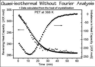
The cold crystallization of PET was analyzed by running the series of quasiisothermal experiments at 388 K and evaluated as shown in Fig. A.13.3. The reversing Cp ( ) decreases, as expected from the lower Cp of the crystallized sample. The same decrease can be calculated from the integral of the total heat-flow rate over

Fig. A.13.3

time, the latent heat, and used to estimate the heat capacity as sum of contributions of amorphous and crystalline fractions (+). As expected, both data sets agree, but the reversing heat capacity has smaller fluctuations. The imbalance in Cp ( ) is calculated from Eq. (3). It is a measure of the kinetics of the cold crystallization by assessing the evolution of the latent heat. It speeds up until about 12 min into the quasi-isothermal experiment, and then slows to completion at about 60 min.

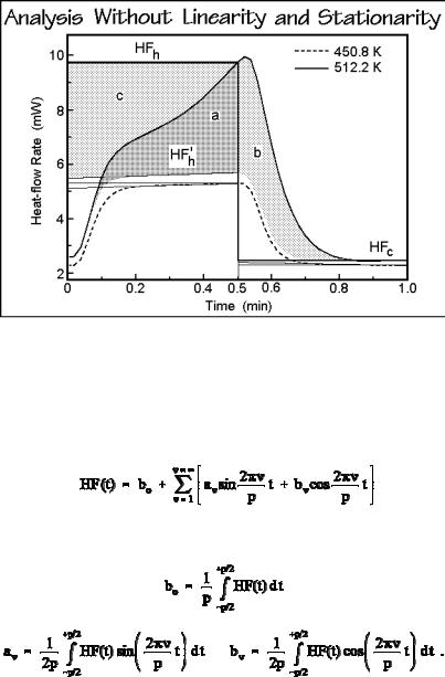
An example of modulation cycles of PET at 450.8 K (before major melting) and 512.2 K (at the melting peak) is displayed in Fig. A.13.4. The measurements at 450.8 K reach steady state on both, heating and cooling, the ones at 512.2 K, only on cooling. On heating at 512.2 K, the heating is interrupted at 0.5 min by the cooling cycle, but melting continues from (a) to (b) despite of the beginning of cooling. Comparing the heat-flow rates to the data taken at 450.8 K allows an approximate separation of the melting, as marked by the shadings. Comparing the heating and cooling segments suggests an approximate equivalence of (b) and (c), so that the

840 Appendix 13–Description of Sawtooth-modulation Response

__________________________________________________________________

Fig. A.13.4

marked HFh accounts for practically all irreversible melting (a + b) and the reversible heat capacity. The cooling segment when represented by HFc, contains almost no latent heat, and similarly, the heat-flow rate HFh' is a measure of the heat-flow rate on heating without latent heat.

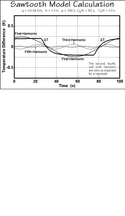
Turning to the analyses of periodic functions, such as the modulated heat-flow rate HF(t), using Fourier series, one can find in any mathematics text the derivation of the following recursion formula [2]:

(4)

where is a running integer starting from 1, and the constant bo and the maximum amplitudes a and b are given by:

(5)

(6)

The data deconvolution for = 1 starts with the evaluation of bo, equal to the total heat-flow rate, <HF(t)>, and is completed with determination of a1 =2<HFsin(t)> and the value of b1 = 2<HFcos(t)>, the first harmonic terms of the Fourier series described in Sect. 4.4.3. A sinusoidal curve has no further terms in Eq. (4). Higher harmonics need to be considered if the sliding average bo is not constant over the modulation

__________________________________________________________________

±0.05 K sinusoidal modulation amplitude. The main part of the melting of C50H102 is clearly reversible. The standard DSC shows the expected broadening in the melting peak due to the lag of the instrument. The extrapolated onset of the melting temperature, as defined for the standard DSC in Fig. 4.62, agrees with point D of the quasi-isothermal TMDSC. Lissajous figures of the heat-flow rate plotted versus the sample temperature in Fig. A.13.12 for points A to D indicates that the final heat of fusion is too large for complete melting in one modulation cycle, as was also seen for the reversibly melting indium in Fig. 4.109, 4.134 and 4.135. At point A in Figs. A.13.11 and A.13.12 the reversing heat-flow rate is already considerably larger

Fig. A.13.12

than expected for the crystals as can be judged from the Lissajous figure for the melt at the highest temperature indicated. The deviation from a perfect ellipse indicates further, that the response is not symmetric in the heating and cooling cycle. The melting and crystallization have either different rates over the modulation cycle, or the mechanisms are more complicated than just melting and crystallization, they may involve, for example, growth of metastable crystals on cooling, followed by annealing to stabler crystals before reaching their melting temperature. The missing area of the explained by the major melting which is not completed within the modulation cycle, as seen at temperatures C and D. Even if there were enough time within the modulation cycle to complete melting and crystallization, the simulated response of a single reversible cycle of melting followed by crystallization in Fig. A.13.13 shows that a straight-forward analysis of the heat-flow rate HF(t), as outlined in Sect. 4.4.3, would not lead to a good representation of the melting and crystallization process. The main reason for the deviations is the nonstationary response.

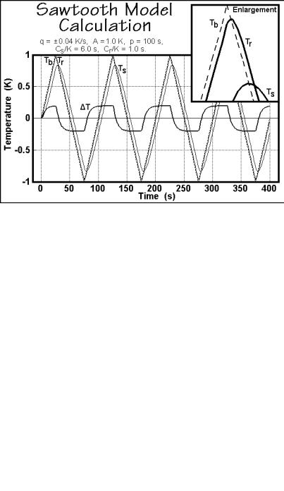
The sawtooth modulation shown in Fig. A.13.14 allows an easy interpretation of the actual data for a similar pentacontane sample as in Figs. A.13.11 and A.13.12.