Thermal Analysis of Polymeric Materials

__________________________________________________________________

Fig. A.10.4

To accomplish and exceed the fast calorimetry just suggested, one can turn to integrated circuit calorimetry. The measuring methods may be modulated calorimetry, such as AC calorimetry or the 3 -method [7,8], thin-film calorimetry as shown in Fig. A.10.4, or may involve standard heating or cooling curves as well as DSC configurations as illustrated in Chap. 4. Modern versions of such fast heating calorimeters are based on silicon-chip technology for measuring heat flow using thermopiles integrated in the chip and resistors for heating. Increasingly more numerous chips have become available based on free-standing membranes of SiNx, produced by etching the center of a properly coated Si-chip, as illustrated in Figs. A.10.5 and A.10.6, which contain each a schematic of the calorimeter.

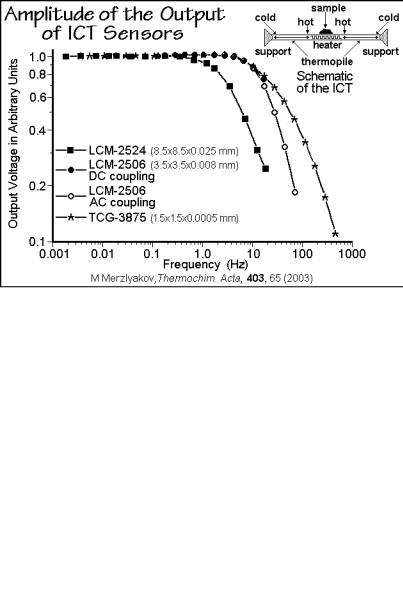
Figure A.10.5 illustrates the performance of several integrated circuit thermopiles, ICT, by Xensor Integration. The calibration without sample shows a constant output voltage of the sensor, decreasing at higher frequency, depending on the membrane used. The phase-angle response shows an analogous change at higher frequency. A linearity-check revealed that dynamic heat capacity measurements should be possible over the frequency range of 1 mHz to 100 Hz, compared to the 0.1 Hz limit typical for TMDSC of Sect. 4.4. This allows to analyze nanogram samples deposited from solution on the position shown in Fig. A.10.5. Similar chips for the measurements of heat capacity of samples of below 1 mg, contained in small aluminum pans, showed time resolutions well below 1 s when using heat-pulses [9].

Finally, Fig. A.10.6 illustrates the change in the crystallization rate when going from slow cooling, measured by standard DSC, to fast standard DSC, and to, ultimately, a chip calorimeter with 5,000 K s 1 (300,000 K min 1) [10]. The cooling rates were varied over five orders of magnitude by using different calorimeters. The cooling rates in the figure from right to left are: for 4 mg in a standard DSC, 0.02, 0.03, 0.08, 0.2, and 0.3 K s 1; for 0.4 mg in a fast DSC: 0.3, 0.8, 3, and 8 K s 1; for

828 Appendix 10–Extreme DTA and DSC

__________________________________________________________________

Fig. A.10.5

Fig. A.10.6

0.1 g in an IC calorimeter as shown in the sketch: 0.45, 0.9, 2.4, and 5 kK s 1. In this chip-calorimeter, the SiNx film, supported by the Si-chip frame was about 500 nm thick. The cooling was achieved by overcompensating the heater power with a cooled purge gas. The heating experiments could also be used to study the reorganization, as discussed in Sect. 6.2.

__________________________________________________________________

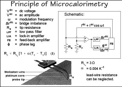
The principle of microcalorimetry is illustrated with Fig. A.10.7 ( TA™ of TA Instruments, Inc.). The tip of an atomic force microscope, AFM, is replaced by a Ptwire that can be heated and modulated, as is illustrated in detail with Fig. 3.96. A typical resolution is about 1.0 m with heating rates up to 1,000 K min 1. A temperature precision of ±3 K and a modulation frequency up to 100 kHz has been reached. The figure shows the control circuit for localized thermal analysis. In this case the probe contacts the surface at a fixed location with a programmed force, controlled by the piezoelectric feedback of the AFM. A reference probe is attached next to the sample probe with its tip not contacting the sample, allowing for

Fig. A.10.7

differential measurements. Equal dc currents are applied to both probes and are controlled by the temperature-feedback circuit to achieve a constant heating rate. The temperature of the sample, Ts, can be determined, after calibration from the resistance of the probe. Since the resistance of platinum has an almost linear dependence on temperature between 300 and 600 K, Rs, can be expressed as shown in Fig. A.10.7, where Rso and are the resistance and the temperature coefficient of the platinum wire at To. The resistance of all lead wires and the heavy Wollaston-portion of the sensor are neglected. Their resistance is small when compared to the V-shaped platinum tip. In addition to the dc current, an ac current can be superimposed on the tip to obtain a temperature-modulation. The dc difference of power between the sample and reference probes is determined by measuring the dc voltage difference between two probes after low-pass filtering (LPF) and the ac voltage difference is measured by the lock-in amplifier (LIA). This arrangement permits an easy deconvolution of the underlying, dc and the reversing ac effects (see also Sect. 4.4). An example which illustrates a qualitative local thermal analysis with a microcalorimeter is given in Fig. 3.97, the limits were probed in [12].

830 Appendix 10–Extreme DTA and DSC

__________________________________________________________________

References for Appendix 10

1.Wunderlich B (2000) Temperature-modulated Calorimetry in the 21st Century. Thermochim Acta 355: 43–57.

2.White GK (1979) Experimental Techniques in Low Temperature Physics. Clarendon, Oxford, 3rd edn.

3.Gmelin E (1987) Low-temperature Calorimetry: A particular Branch of Thermal Analysis. Thermochim Acta 110: 183–208.

4.Lounasma OV (1974) Experimental Principles and Methods below 1 K. Academic Press, London; see also Bailey CA, ed (1971) Advanced Cryogenics. Plenum Press, New York.

5.Wu ZQ, Dann VL, Cheng SZD, Wunderlich B (1988) Fast DSC Applied to the Crystallization of Polypropylene. J Thermal Anal 34: 105–114.

6.Pijpers TFJ, Mathot VBF, Goderis B, Scherrenberg RL, van der Vegte EW (2002) Highspeed Calorimetry for the Study of the Kinetics of (De)vitrification, Crystallization, and Melting of Macromolecules. Macromolecules 35: 3601–3613.

7.Jeong Y-H (2001) Modern Calorimetry: Going Beyond Tradition. Thermochim. Acta

377:1–7.

8.Jung DH, Moon IK, Jeong Y-H (2003) Differential 3 Calorimeter. Thermochim. Acta

403:83–88.

9.Winter W, Höhne WH (2003) Chip-calorimeter for Small Samples. Thermochim. Acta

403:43–53.

10.Adamovsky SA, Minakov AA, Schick C (1003) Thermochim. Acta 403: 55–63. Figure modified from a presentation at the 8th Lähnwitz Seminar of 2004, courtesy of Dr. C. Schick.

11.Moon I, Androsch R, Chen W, Wunderlich B (2000) The Principles of Micro-thermal Analysis and its Application to the Study of Macromolecules. J Thermal Anal and Calorimetry 59: 187–203.

12.Buzin AI, Kamasa P, Pyda M, Wunderlich B (2002) Application of Wollaston Wire Probe for Quantitative Thermal Analysis, Thermochim Acta, 381, 9–18.

__________________________________________________________________

The use of the corrections B in Fig. A.11.2 needs two calibration runs of the DSC of Fig. 4.54. The heat capacities of the calorimeter platforms, Cspl and Crpl, and the resistances to the constantan body, Rspl and Rrpl, must be evaluated as a function of temperature. First, the DSC is run without the calorimeters, next a run is done with sapphire disks on the sample and reference platforms without calorimeter pans. From the empty run one sets a zero heat-flow rate for .s and .r. This allows to calculate the temperature-dependent time constants of the DSC, written as s = CsplRspl andr = CrplRrpl, and calculated from the equations in the lower part of Fig. A.11.2. For the second run, the heat-flow rates are those into the sapphire disks, known to be mcpq, as suggested in Figs. 4.54 and 4.70. The heat-capacity-correction terms are zero in this second calibration because no pans were used. From these four equations, all four platform constants can be evaluated and the DSC calibrated.

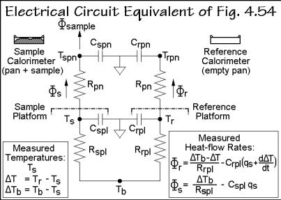
As the next step, the effect of the pans must be considered. The differences between sample and reference pan cause similar heat-flow problems as the platforms and can be assessed by the diagram of Fig. A.11.3. The dash-dotted lines indicate the

Fig. A.11.3

sample and reference platforms from which .s and .r, contained in Eq. (3), enter into

the calorimeters. The heat-flow rate into the sample, .sample, however, is modified by the heat resistance between pan and platform, Rpn, and the heat capacity of the pan

Cspn. The actual sample temperature inside the calorimeter pan, in turn, is not Ts, but the temperature Tspn. For the reference side, one assumes the same thermal resistance Rpn, but because of the possibly different mass of the reference pan, a different Crpn. Assuming further that the reference calorimeter is empty, as is the usual operation

procedure, there is no .reference.

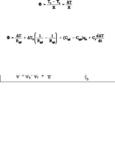
Using the two measured temperature differences T and Tb listed in Fig. A.11.3 and inserting them into the heat-flow rate expressions of sketch B of Fig. A.11.2 yields the two heat-flow rates of Fig. A.11.3 and their difference, expressed in

834 Appendix 11–Online Correction of the Heat-flow Rate

__________________________________________________________________

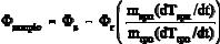
Eq. (2), above. To obtain the actual heat-flow rate into the sample, .sample, one has to compute the heat-flow rates into the two pans. Since both pans are out of the same

material Cspn = mspn cpan and Crpn = mrpn cpan, where cpan is the specific heat capacity of the pan material and m represents the corresponding mass. Since all .r goes into the

empty pan, one can use its value to compute .sample:

(3)

Insertion of the measured values for .s and .r, contained in Fig. A.11.3, leads to an

overall equation for .sample. The needed sample and reference pan temperatures in Eq. (3) can be calculated with some simple assumptions about the contact resistance

between pan and platform Rpn [2]: Tspn = Ts .s Rpn and Trpn = Tr .r Rpn. The commercial software includes typical values derived from data given in [5],

considering geometry, purge gas, and pan construction.

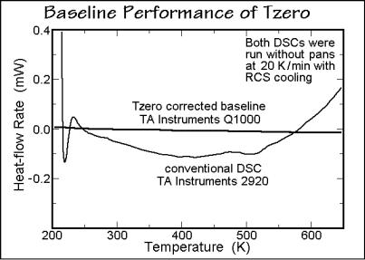
To summarize, the correction for asymmetry of the measuring platforms in Fig. 4.54 due to their thermal resistances and their heat capacities with Eq. (3) eliminates the main effect of the baseline curvature with temperature, as is shown in Fig. A.11.1. Further corrections include the mass differences of the pans and the thermal resistance between calorimeters and measuring platforms.

Remaining problems are the temperature gradients within the sample and their changes on heating or cooling, deformations of the sample pan and the accompanying changes in contact resistances which occur when samples expand or shrink. Also, the position of the calorimeters should be fixed and must not be altered during measurement, as can happen by vibrations or mechanical shocks. Changes of heat transfer due to radiation can be caused by fingerprints on calorimeters, platforms, and furnace cavity since fingerprints are easily converted at high temperatures to carbon specks with higher emissivity and absorptivity. Once cleaned, it is helpful to use dust-free and clean nylon gloves and to touch the calorimeters with tweezers only. The purge gas must not change in flux and pressure from the calibration and must not develop turbulent flow or convection currents. Finally, the room temperature must not fluctuate and set up changing temperature gradients within the DSC. Avoidance of all these potential errors is basic to good calorimetry.

References to Appendix 11:

1.Waguespack L, Blaine RL (2001) Design of A New DSC Cell with Tzero™ Technology. Proc 29th NATAS Conf in St. Louis, MO, Sept 24–26, Kociba KJ, Kociba BJ, eds 29: 721–727.

2.Danley RL (2003) New Heat-flux DSC Measurement Technique. Thermochim Acta 395:201–208.

3.Höhne G, Hemminger W, Flammersheim HJ (2003) Differential Scanning Calorimetry, 2nd edn. Springer, Berlin.

4.Holman JP (1976) Heat Transfer, 4th edn. McGraw-Hill, New York, pp 97–102.

5.Madhusudana CV (1996) Thermal Contact Conductance. Springer, New York.

__________________________________________________________________

Derivation of the Heat-flow-rate Equations

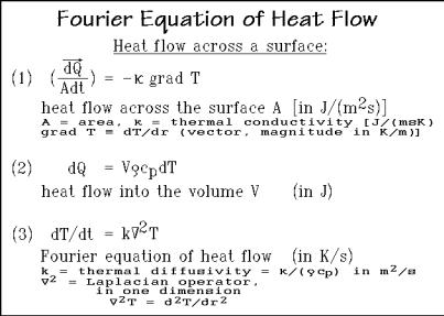
The heat flow across any surface area, A, is given in Fig. A.12.1 by the heat-flow rate per unit area dQ/(Adt) in Eq. (1), a vector quantity in J m 2s 1. It is equal to the negative of the thermal conductivity,1 in J m 1s 1K 1, multiplied by the temperature gradient (dT/dr). Equation (2) represents the differential heat flow into the volume

Fig. A.12.1

V and can be derived from the definition of the heat capacity dQ/dT = mcp. The symbols have the standard meanings; is the density and cp, the specific heat capacity per unit mass, so that m = V .

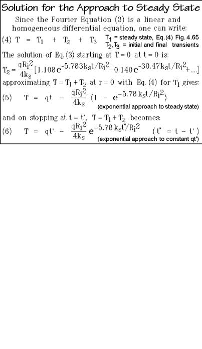
Standard techniques of vector analysis allow to equate the heat flow into the volume V to the heat flow across its surface. This operation leads to the linear and homogeneous Fourier differential equation of heat flow, given as Eq. (3). The letter k represents the thermal diffusivity in m2 s 1, which is equal to the thermal conductivity 1 divided by the density and specific heat capacity. The Laplacian operator is 2 = 2/ x2 + 2/ y2 + 2/ z2, where x, y, and z are the space coordinates. In the present cylindrical symmetry, the Laplacian, operating on temperature T, can be represented as d2T/dr2 reducing the equation to one dimension. Equations (1) (3) form the basis for the further mathematical treatment of differential thermal analysis, as is given, for example by Ozawa T (1966) Bull. Chem. Soc. Japan 39: 2071.

The superposition principle is obeyed by the solutions of Eq. (3), i.e., the combined effect of a number of causes acting together is the sum of the effects of the causes acting separately. This allows the description of phase transitions by evaluating several separate solutions and adding them, as suggested in Fig. A.12.2. For a modeling of the glass transition in a DSC with Ri = 4 mm, see Fig. A.12.3.