Thermal Analysis of Polymeric Materials

__________________________________________________________________

Fig. A.3.2

angle. Equation (1) in Fig. A.3.3 combines the equations of Fig. A.3.2. The analysis of Eq. (1) is drawn in form of a polar diagram of the intensity of the scattered light. The length of each of the lines of the doughnut-shaped, three-dimensional figure indicates the intensity of scattered light in the direction of the line, i.e., the largest intensity is normal to the vibration direction z of the induced dipole, the smallest is zero, seen along direction z. All other intensities change as indicated in the figure.

Fig. A.3.3

808 Appendix 3–Derivation of the Rayleigh Ratio

__________________________________________________________________

The change which occurs when going from the scattering of the polarized light, just derived in Eq. (1), to unpolarized light is also shown in Fig. A.3.3 with Eq. (2). The derivation of the equation involves the addition of the scattering intensities from two identical light beams traveling in the same direction, but being polarized at right angles in the xz and xy planes. Using the simple relationship sin2"z cos2"y = cos2 and division by 2, because each polarized component contributes only half the total scattered light, leads from Eq. (1) to Eq. (2).

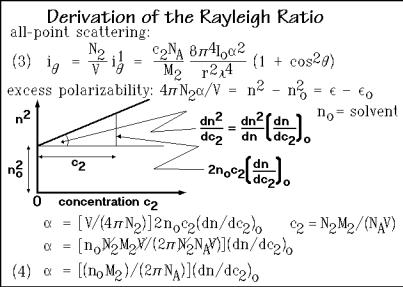
The final equation adds the intensities from all scattering points (assuming no interference) as shown in Eq. (3) of Fig. A.3.4. The value N2 is the total number of scattering centers, and V is the volume in which the scattered light is generated. The last part of Eq. (3) is linked to the experimentally available quantities. The measured quantities and known constants are expressed by introducing the concentration c2 in Mg m 3, Avogadro’s number NA = 6.02×1023, and the molar mass M2. The subscript 2 is used for quantities referring to macromolecules.

To summarize the derivation given so far, Eq. (1) explains already the strong wavelength dependence of the scattered light (fourth power, blue light scatters more than red), indicates that scattering is zero in direction of the z-axis (sin "z = 0), and shows rotational symmetry about the z-axis. Next, going from Eq. (1) for the scattering of plane-polarized light to unpolarized light is done with Eq. (2). The addition of the second beam of light for Eq. (2) superimposes an identical symmetry of scattered light about the y-axis, but with opposite polarization. At = 90° the angular dependence of Eq. (2) is 1.0 and the scattered light changes in polarization on going from the direction of the y-axis to the direction of the z-axis. At = 0 and 180° the last factor of Eq. (2) is 2, its maximum, accounting for the strong forward and reverse scattering. Finally, adding scattered light from all centers leads to Eq. (3). Because one assumed no interference between the different, coherently

Fig. A.3.4

__________________________________________________________________

scattered rays, Eq. (3) is limited to dilute solutions. Experiments at higher concentration have to be extrapolated to infinite dilution.

The next step of interpretation of Eq. (3) is the development of an expression for the excess polarizability, , caused by the dissolution of the polymer in the solvent. This is done by remembering that the polarizability at the frequency of light is related to the squares of the refractive index, n2 (as well as the permittivity, the dielectric constant, ). The connection between and n is written at the top of Fig. A.3.4. Its background can be found in any physical chemistry text. Assuming the square of the refractive index changes linearly with concentration, one can draw the sketch in the figure. The refractive index no refers to the pure solvent, while n is the refractive index of the solution of concentration c2.

The angle and amplitude of the change of the refractive index with concentration can next be changed to a differential expression at concentration zero. Note that at zero concentration dn2/dc2 = 2no(dn/dc2)o is a quantity that can be measured with a differential refractometer using a series of concentrations of the polymer to be analyzed and extrapolation to concentration zero. Naturally, the solution must change sufficiently in n with increasing concentration to achieve measurable light scattering. The polarizability is needed for the evaluation of Eq. (3). The insertion of the expression for the concentration c2, and the final simplification to Eq. (4) is shown at the bottom of Fig. A.3.4.

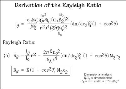
The insertion of Eq. (4) into Eq. (3) and the simplification of the expression for i is indicated at the top of Fig. A.3.5. The Rayleigh ratio of the light which is scattered into the direction is the main outcome of the present derivation. It is shown at the bottom as Eq. (5). The Rayleigh ratio eliminates the influence of the measuring distance r and the incident light intensity. Both are instrumental calibration parameters. When all of the constants of the to-be-analyzed system are

Fig. A.3.5

__________________________________________________________________

Neural Network Predictions

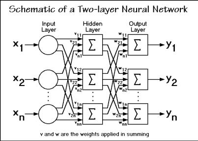
Neural net computation is a technique of data handling that is quickly gaining importance. A neural network can be thought of as a mathematical function with generalized estimation and prediction capabilities. It is a computational system made up of a number of simple, yet highly connected, layered processing elements called nodes or neurons. The neurons process information by their dynamic response to external information.

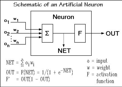
Neural networks, as the name implies, were originally biologically inspired to perform in a manner analogous to the basic functions of neurons. The network is specified by its architecture, transfer functions, and learning laws. Figure A.4.1 illustrates that the input from the net to a given neuron (NET), is the sum of the inputs, oi, each multiplied with its corresponding weight, wi. Before the NET is passed on to the subsequent network layers, it is multiplied with a nonlinear transfer function, F, as indicated in the figure. The architecture of a simple network is given in the Fig. A.4.2. If needed, additional layers can be added to the network, complicating the schematic of the structure.

Before the network can be used, it must undergo a learning step. The network learns in a computation-intensive step by establishing the weights that, when applied to the inputs of the nodes, will yield the required output. Note that the derivative of F(NET) with respect to the output, OUT, is rather simple in the chosen example (F’ in Fig. A.4.1). Since only the learning step of the network takes a considerable amount of computer time, it is possible to have the learning done on a larger and faster computer and transfer the once established weights to a desktop computer for everyday use in one’s own and other laboratories. One may also speculate that it may

Fig. A.4.1

__________________________________________________________________

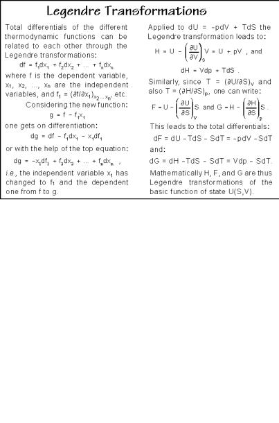
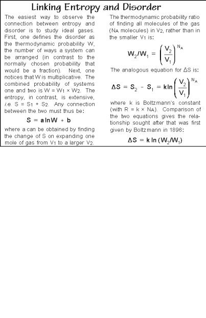
Legendre Transformations, Maxwell Relations, Linking Entropy and Probability, and Derivation of dS/dt

The title topics are represented in the Figs. A.5.1–4, shown below:

Fig. A.5.1

Fig. A.5.2

814 Appendix 5–Thermodynamics Calculations

__________________________________________________________________

Fig. A.5.3

Fig. A.5.4

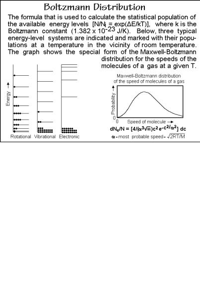
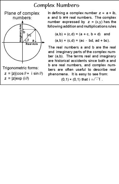
Boltzmann Distribution, Harmonic Vibrations, Complex

Numbers, and Normal Modes

The title topics are represented in the Figs. A.6.1–4, shown below:

Fig. A.6.1

Fig. A.6.2

816 Appendix 6–Boltzmann Distribution, Complex Numbers, Vibrations

__________________________________________________________________

Fig. A.6.3

Fig. A.6.4