

Thermal Analysis of Polymeric Materials
.pdf56 1 Atoms, Small, and Large Molecules
__________________________________________________________________
Fig. 1.58
forward scattering seen in Fig. 1.58 since all scattered light adds with the same phase as the incoming light. For the shape determination, P must be known quite precisely since the changes between discs, rods, random coils, spheres and other shapes can be quite small, as seen in the figure.
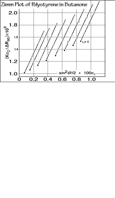
Typical light-scattering data for polystyrene in butanone are plotted in Fig. 1.59 in a method which was suggested originally by Zimm [20,21]. The abscissa is
Fig. 1.59
1.4 Size and Shape Measurement |
57 |
__________________________________________________________________
Fig. 1.60
proportional to the functional shape-dependence for a random coil, sin2 /2, added to the concentration c2, multiplied with an arbitrary constant k = 100 (arbitrarily chosen so that the points are well separated). Next, in Fig. 1.60, all sets of data at the same scattering angle are extrapolated to zero concentration. The slopes of these lines are largely parallel. Extrapolating in addition to zero angle, as shown in Fig. 1.61, yields the so-called Zimm plot. The slope of the line of zero concentration is proportional
Fig. 1.61
58 1 Atoms, Small, and Large Molecules
__________________________________________________________________
to the mean square of the distance of the chain elements from their center of gravity (<s2>½ = 46 nm); the slope of the line at zero scattering angle, which is proportional to the second virial coefficient (A2 = 1.29×10 4 m3 mol/kg2); and the common intercept at zero concentration and angle, yields the inverse of the mass-average molar mass (Mw = 1,030,000 Da).
Finally, the integration of the Rayleigh ratio over all angles can make the connection of the scattered light in direction to the turbidity , mentioned at the beginning of this section. The result is K/R90 = H/ with the constant H given by:
This completes the discussion of light scattering. These data were the source of much of the information discussed in Sect. 1.3. Next, a series of other, somewhat simpler characterization techniques is discussed which can be used to determine average molar masses. With size-exclusion chromatography and ultracentrifugation, distributions can also be assessed.
1.4.3 Freezing Point Lowering and Boiling Point Elevation
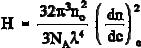
The ereezing point lowering and boiling point elevation of a low-molar-mass solvent due to the presence of a solute are colligative properties as described in Fig. 1.52, i.e., they are independent of the type of solute. One can thus use these properties to determine the molar mass of a polymeric solute. Figure 1.62 shows the appropriate equations and pressure-temperature phase diagram. The polymer mole fraction x2 is expressed in terms of heat of fusion ( Hf) or evaporation ( Hv), the freezing point lowering or boiling point elevation ( T) and the equilibrium melting or boiling temperatures (Tmo or Tbo). The gas constant R is 8.3143 J K 1 mol 1 and T is the temperature of measurement in kelvins. The equations can be derived easily, as is shown in the final result of Sect. 2.2.5 in Fig. 2.26, below.
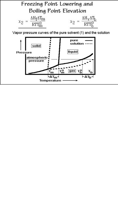
Before the equations of Fig. 1.62 can be applied to experiments, they must be rewritten in terms of the measurable and known quantities, as is illustrated in Fig. 1.63. First the mole fraction is expressed in terms of concentration c2 in g per kg of solvent (note the difference from the c2 used in light scattering). On insertion for x2, the heats of transitions are conveniently changed to the latent heats (J per kg of solvent). The mole fractions are available after the completed experiment.
The data treatment is illustrated in Fig. 1.64. Since ideal behavior is only expected at infinite dilution, the indicated extrapolation is necessary. This applies especially to macromolecular solutes. A list of values for RT2 L 1 for different solvents is shown at the bottom of the figure. It should be looked at in terms of the dimensionless variables T/T, the change in transition temperature in multiples of absolute temperature, and L/RTm,bo, the entropies of transition in multiples of R. The smaller the entropy change (larger RTm,bo/L), the larger is T/T. Plastic crystal forming liquids, such as cyclohexane and camphor have a much smaller entropy of isotropization than rigid crystals of similar molecular structure (see Chap. 5) and are thus good solvents for freezing-point lowering experiments. Since the entropy of
1.4 Size and Shape Measurement |
59 |
__________________________________________________________________
Fig. 1.62
evaporation is always larger than the entropy of fusion and does not change much for different solvents since all follow Trouton’s rule (see Sect. 2.5.7), one needs higher precision of the thermometry for the determination of molar mass by boiling point elevation.
Figure 1.65 illustrates a differential ebulliometer for the measurement of boiling point elevations. This ebulliometer gives the precision which is required for
Fig. 1.63
60 1 Atoms, Small, and Large Molecules
__________________________________________________________________
Fig. 1.64
polymeric solutes. The upper bank of thermocouple reference junctions is kept at the boiling temperature of the pure solvent by being in the reflux stream of the condensed vapor (at Tbo). The measuring thermocouples are kept at the boiling point of the solution by having the solution flowing across their surface from the exit of the Cottrell pump that works like a percolator. The overheating, possible in the reservoir of solution, is thus kept low. There is no commercial ebulliometer, perhaps because
Fig. 1.65
1.4 Size and Shape Measurement |
61 |
__________________________________________________________________
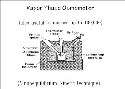
of the success of an empirical method of measuring the differential evaporation and condensation of solvent vapor from pure solvent and from solution, the vapor phase osmometer shown in Fig. 1.66. With the indicated syringe a pure solvent drop is
Fig. 1.66
placed on one thermistor probe, and a solution drop on the other. The chamber is kept at the vapor pressure of the solvent, so that the measured T is proportional to the rate of excess condensation of solvent vapor on the solution droplet. Since the rates are not only dependent on the lower vapor pressure at the surface of the solution droplet, but also on the rates of mass diffusion and heat conduction, T must be calibrated with known standards.
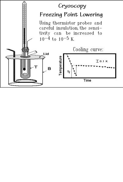
Figure 1.67 shows a schematic of a simple, but effective set-up for cryoscopy, the method for the measurement of the freezing point lowering. Cryoscopy is perhaps the easiest of the molar mass determinations. The main prerequisites are a good temperature control and uniformity, corrections for the common supercooling observed on crystallization, and the usual extrapolation to infinite dilution. The thermodynamic equations are derived in Sect. 2.2.5, together with the equations needed for the ebulliometry.
The molar mass data for six typical polyethylene samples are listed in Fig. 1.68 [22]. They permit judgement of the routine precision for such experiments. Only ebulliometry and cryoscopy are absolute methods and need no calibration. Using the greatest possible precision, ebulliometry, vapor phase osmometry, and cryoscopy can be used up to 100,000 Da. Light scattering, also an absolute method, can readily measure up to 10,000,000 Da and give, in addition, information on the shape of the molecules, but may have difficulties with the lowest molar masses. The interaction parameter A2 could, in principle, be extracted from the concentration dependence of light scattering, ebulliometry, and cryoscopy data.
62 1 Atoms, Small, and Large Molecules
__________________________________________________________________
Fig. 1.67
Fig. 1.68
1.4.4 Size-exclusion Chromatography
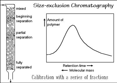
Size-exclusion chromatography, also called by its older designation gel-permeation chromatography, permits the separation of different sizes of molecules by retarding the smaller ones longer than the larger ones while passing over a specially prepared
1.4 Size and Shape Measurement |
63 |
__________________________________________________________________
gel (for the description of gels, see Fig. 3.48, below). Figure 1.69 shows a schematic sketch of the process. The different fractions of the polymer appear at different times at the bottom of the column. The calibration is done with well-known, commercially
Fig. 1.69
available, polymer fractions. Polystyrene is often used, but different polymers may deviate considerably from a polystyrene calibration. Analyzing the emerging fractions with one of the absolute methods discussed above is the best calibration method. After the calibration, a full distribution curve of molecular sizes can be found, as indicated in the figure. This method goes thus far beyond the establishment of an average molar mass or a moment of the distribution as described in Sect. 1.1.3. At least number and mass average and polydispersity should be established. Besides analysis, preparative separation of a sample into narrow molar mass fractions is also possible.
1.4.5 Solution Viscosity
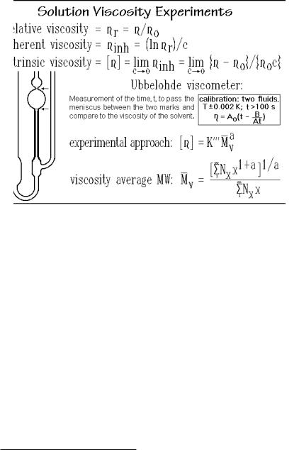
Solution viscosity was already recognized by Staudinger as a useful measure of the size of macromolecules. It is a measure of the extension of the molecule in solution. The larger the extension, the larger should be the contribution to the solution viscosity. Usually it is related empirically to the molar mass, although models have been developed to understand the results. Figure 1.70 shows a drawing of an Ubbelohde capillary viscometer. Constant temperature ±0.002 K and efflux-times above 100 s are required. The viscosity (measured in Pa s = J cm 3 s 1) for a given viscometer is then proportional to the efflux time (see also Chap. 5). The viscometer is calibrated with two known liquids. Measurements are made at different concentrations c2 (in g/100 mL) to extrapolate to zero concentration. Three
64 1 Atoms, Small, and Large Molecules
__________________________________________________________________
Fig. 1.70
commonly given viscosity measures are listed in the figure, where o is the solvent viscosity. The intrinsic viscosity suggests the extrapolation procedure for a measure of the influence of the polymer on the solvent viscosity.
Modeling polymer viscosity starts with calculating the effect of separate, solid spheres immersed in a solvent. The first result was already given by Einstein1 in 1911 [23] ([ ] = 2.5/density of the solute in Mg/m3). The energy dissipated by the spheres at the given concentration c2 each second per unit volume of solution is equal to the intrinsic viscosity. The next step is to go to the freely draining model for which more details are given in the discussion of melt viscosity in Sect. 5.6.6. One assumes that the macromolecule rotates as a whole through the action of the shear-gradient, but entraps no solvent. On summation of the frictional energy over all parts of the molecule assumed to be solid beads. This summation was first done by Debye [24,25], a proportionality to the mean-square end-to-end distance with an expansion factor 2 results in the expression:
[ ] = K <r2> 2 .
At the -temperature, the excluded volume effect is avoided ( = 1.0, see Sect. 1.3.). Making some solvent to rotate with the molecule leads to the equivalent sphere model. In this case one assumes that a certain inner solid sphere of solvent is
1 Albert Einstein (1879–1955), born in Ulm, Germany. He was recognized in his own time as one of the most creative intellects in human history. Einstein studied mathematics and physics at the ETH in Zürich until 1900 when he became a Swiss citizen. In 1905 he earned his Ph.D. from the University of Zürich. The later life was in Berlin (1914–33) and then Princeton, NJ. Nobel Prize for Physics in 1921 (for work on photoelectricity and theoretical physics).
1.4 Size and Shape Measurement |
65 |
__________________________________________________________________
entrapped by the macromolecule and rotates with it in the shear-gradient. The intrinsic viscosity is now decreased to the square-root dependence on the molar mass of the polymer, M2:
[ ] = K M2½ 3 .
Neither the limits of the freely-draining nor the equivalent sphere give, however, the proper proportionality. One uses thus an empirical approach by calibration with standards as indicated in Fig. 1.70. The exponent a is typically fractional, between 0.6 and 0.8. As a result, the viscosity average molar masses are neither of the averages discussed in Sect. 1.4.3. A special average is defined as given in Fig. 1.70. The viscosity average molar mass, written as Mv, is closer to Mw than to Mn, as seen in the last line of the figure.
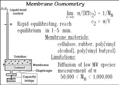
1.4.6 Membrane Osmometry
The osmotic pressure is again a colligative property and leads, thus, to an absolute molar mass and for a distribution of different species, a number-average molar mass, as summarized in Fig. 1.71. The pressure p of the ideal gas law is replaced by the osmotic pressure , w is the total mass dissolved, so that w/M n is the number of moles, n to give the link to pV = nRT.
Measurements became easier with rapidly equilibrating membrane osmometers with servo pressure control. The instrument senses differences in osmotic pressure based on the mass transport through the membrane. The pressure differential between solvent and solution is then controlled by increasing the solution level to hydrostatically counterbalance the osmotic pressure . The success of the osmometry
Fig. 1.71