Thermal Analysis of Polymeric Materials

__________________________________________________________________

2.3.5 Complex Heat Capacity

In general, one can represent a complex number, defined in Fig. A.6.3 of Appendix 6 as z = a + ib, with i = 1. A complex number can also be written as:

(1)

(2)

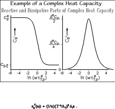
For the description of periodic changes, as in modulated-temperature differential scanning calorimetry [19], TMDSC (see Sect. 4.4), or Fourier analyses, the introduction of complex quantities is convenient and lucid. It must be noted, however, that the different representation brings no new physical insight over the description in real numbers. The complex heat capacity has proven useful in the interpretation of thermal conductivity of gaseous molecules with slowly responding internal degrees of freedom [20] and may be of use representing the slow response in the glass transition (see Sect. 5.6). For the specific complex heat capacity measured at frequency , cp( ), with its real (reactive) part cp ( ) and the imaginary part icp ( ), one must use the following equation to make cp ( ), the dissipative part,

positive:

(3)

The real quantities of Eq. (3) can then be written as:

(4)

(5)

where eT,p is the Debye relaxation time of the system. The reactive part cp ( ) of cp( ) is the dynamic analog of cpe, the cp at equilibrium. Accordingly, the limiting cases of a system in internal equilibrium and a system in arrested equilibrium are, respectively:

(6)

(7)

The internal degree of freedom contributes at low frequencies the total equilibrium contribution, ecp, to the specific heat capacity. With increasing , this contribution decreases, and finally disappears.

The limiting dissipative parts, cp ( ), without analogs in equilibrium thermodynamics, are:

(8)

(9)

118 2 Basics of Thermal Analysis

__________________________________________________________________

so that the dissipative part disappears in internal equilibrium ( eT,p 0) as well as in

arrested equilibrium ( eT,p ). Figure 2.43 illustrates the changes of cp ( ) and cp ( ) with eT,p.

Fig. 2.43

The dissipative heat capacity cp ( ) is a measure of is, the entropy produced in nonequilibrium per half-period of the oscillation T(t) Te:

(10)

2.3.6 The Crystallinity Dependence of Heat Capacity

Several steps are necessary before heat capacity can be linked to its various molecular origins. First, one finds that linear macromolecules do not normally crystallize completely, they are semicrystalline. The restriction to partial crystallization is caused by kinetic hindrance to full extension of the molecular chains which, in the amorphous phase, are randomly coiled and entangled. Furthermore, in cases where the molecular structure is not sufficiently regular, the crystallinity may be further reduced, or even completely absent so that the molecules remain amorphous at all temperatures.

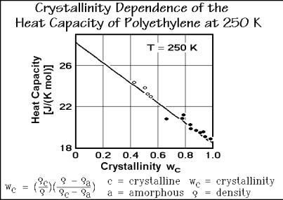
The first step in the analysis must thus be to establish the crystallinity dependence of the heat capacity. In Fig. 2.44 the heat capacity of polyethylene, the most analyzed polymer, is plotted as a function of crystallinity at 250 K, close to the glass transition temperature (Tg = 237 K). The fact that polyethylene, [(CH2 )x], is semicrystalline implies that the sample is metastable, i.e., it is not in equilibrium. Thermodynamics

__________________________________________________________________

Fig. 2.44

requires that a one-component system, such as polyethylene, can have two phases in equilibrium at the melting temperature only (phase rule, see Sect. 2.5).

One way to establish the weight-fraction crystallinity, wc, is from density measurements (dilatometry, see Sect. 4.1). The equation is listed at the bottom of Fig. 2.44 and its derivation is displayed in Fig. 5.80. A similar equation for the volume-fraction crystallinity, vc, is given in the discussion of crystallization in Sect. 3.6.5 (Fig. 3.84). Plotting the measured heat capacities of samples with different crystallinity, often results in a linear relationship. The plot allows the extrapolation to crystallinity zero (to find the heat capacity of the amorphous sample) and to crystallinity 1.0 (to find the heat capacity of the completely crystalline sample) even if these limiting cases are not experimentally available.

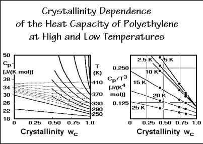
The graphs of Fig. 2.45 summarize the crystallinity dependence of the heat capacity of polyethylene at high and low temperatures. The curves all have a linear crystallinity dependence. At low temperature the fully crystalline sample (wc = 1.0) has a T3 temperature dependence of the heat capacity up to 10 K (single point in the graph), as is required for the low-temperature limit of a three-dimensional Debye function. One concludes that the beginning of the frequency spectrum is, as also documented for diamond and graphite in Sect. 2.3.4, quadratic in frequency dependence of the density of vibrational states, ( ). This 2-dependence does not extend to higher temperatures. At 15 K the T3-dependence is already lost. The amorphous polyethylene (wc = 0) seems, in contrast, never to reach a T3 temperature dependence of the heat capacity at low temperature. Note that the curves of the figure do not even change monotonously with temperature in the Cp/T3 plot.

As the temperature is raised, the crystallinity dependence of the heat capacity becomes less; it is only a few percent between 50 to 200 K. In this temperature range, heat capacity is largely independent of physical structure. Glass and crystal

120 2 Basics of Thermal Analysis

__________________________________________________________________

Fig. 2.45

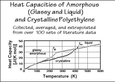
have almost the same heat capacity. This is followed again by a steeper increase in the heat capacity of the amorphous polymer as it undergoes the glass transition at 237 K. It is of interest to note that the fully amorphous heat capacity from this graph agrees well with the extrapolation of the heat capacity of the liquid from above the melting temperature (414.6 K).

Finally, the left curves of Fig. 2.45 show that above about 260 K, melting of small, metastable crystals causes abnormal, nonlinear deviations in the heat capacity versus crystallinity plots. The measured data are indicated by the heavy lines in the figure. The thin lines indicate the continued additivity. The points for the amorphous polyethylene at the left ordinate represent the extrapolation of the measured heat capacities from the melt. All heat capacity contributions above the thin lines must thus be assigned to latent heats. Details of these apparent heat capacities yield information on the defect structure of semicrystalline polymers as is discussed in Chaps. 4–7.

Figure 2.46 illustrates the completed analysis. A number of other polymers are described in the ATHAS Data Bank, described in the next section. Most data are available for polyethylene. The heat capacity of the crystalline polyethylene is characterized by a T3 dependence to 10 K. This is followed by a change to a linear temperature dependence up to about 200 K. This second temperature dependence of the heat capacity fits a one-dimensional Debye function. Then, one notices a slowing of the increase of the crystalline heat capacity with temperature at about 200 to 250 K, to show a renewed increase above 300 K, to reach values equal to and higher than the heat capacity of melted polyethylene (close to the melting temperature). The heat capacity of the glassy polyethylene shows large deviations from the heat capacity of the crystal below 50 K (see Fig. 2.45). At these temperatures the absolute value of the heat capacity is, however, so small that it does not show up in Fig. 2.46. After

__________________________________________________________________

Fig. 2.46

the range of almost equal heat capacities of crystal and glass, the glass transition is obvious at about 240 K. In the melt, finally, the heat capacity is linear over a very wide range of temperature.

2.3.7 ATHAS

The quite complicated temperature dependence of the macroscopic heat capacity in Fig. 2.46 must now be explained by a microscopic model of thermal motion, as developed in Sect. 2.3.4. Neither a single Einstein function nor any of the Debye functions have any resemblance to the experimental data for the solid state, while the heat capacity of the liquid seems to be a simple straight line, not only for polyethylene, but also for many other polymers (but not for all!). Based on the ATHAS Data Bank of experimental heat capacities [21], abbreviated as Appendix 1, the analysis system for solids and liquids was derived.

For an overall description, the molecular motion is best divided into four major types. Type (1) is the vibrational motion of the atoms of the molecule about fixed positions, as described in Sect. 2.3.3. This motion occurs with small amplitudes, typically a fraction of an ångstrom (or 0.1 nm). Larger systems of vibrators have to be coupled, as discussed in Sect. 2.3.4 on hand of the Debye functions. The usual technique is to derive a spectrum of normal modes as described in Fig. A.6.4, based on the approximation of the motion as harmonic vibrators given in Fig. A.6.2.

The other three types of motion are of large-amplitude. Type (2) involves the conformational motion, described in Sect. 1.3.5. It is an internal rotation and can lead to a 360o rotation of the two halves of the molecules against each other, as shown in Fig. 1.37. For the rotation of a CH3-group little space is needed, while larger segments of a molecule may sweep out extensive volumes and are usually restricted

122 2 Basics of Thermal Analysis

__________________________________________________________________

to coupled rotations which minimize the space requirement. Backbone motions which require little additional volume within the chain of polyethylene are illustrated by the computer simulations in Sect. 5.3.4.

The last two types of large-amplitude motion, (3) and (4), are translation and rotation of the molecule as a whole. These motions are of little importance for macromolecules since a large molecule concentrates only little energy in these degrees of freedom. The total energy of small molecules in the gaseous or liquid state, in contrast, depends largely on the translation and rotation.

Motion type (1) contributes R to the heat capacity per mole of vibrators (when excited, see Sect. 2.3.3 and 2.3.4). Types (2–4) add only R/2, but may also need some additional interand intramolecular potential energy contributions, making particularly the types (3) and (4) difficult to assess. This is at the root of the ease of the link of macromolecular heat capacities to molecular motion. The motion of type

(1) is well approximated as will be shown next. The motion of type (2) can be described with the conformational isomers model, and more recently by empirical fit to the Ising model (see below). The contribution of types (3) and (4), which are only easy to describe in the gaseous state (see Fig. 2.9), is negligible for macromolecules.

The most detailed analysis of the molecular motion is possible for polymeric solids. The heat capacity due to vibrations agrees at low temperatures with the experiment and can be extrapolated to higher temperatures. At these higher temperatures one can identify deviations from the vibrational heat capacity due to beginning large-amplitude motion. For the heat capacities of the liquids, it was found empirically, that the heat capacity can be derived from group contributions of the chain units which make up the molecules, and an addition scheme was derived. A more detailed model-based scheme is described in Sect. 2.3.10.

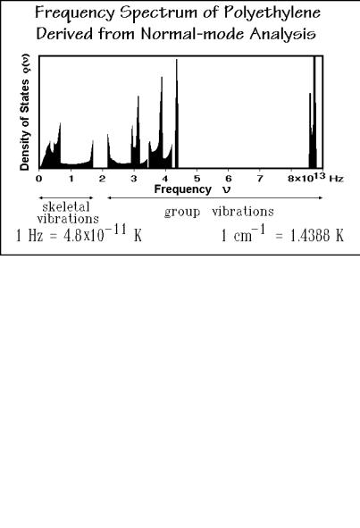
After the crystallinity dependence has been established, the heat capacity of the solid at constant pressure, Cp, must be changed to the heat capacity at constant volume Cv, as described in Fig. 2.31. It helps in the analysis of the crystalline state that the vibration spectrum of crystalline polyethylene is known in detail from normal mode calculations using force constants derived from infrared and Raman spectroscopy. Such a spectrum is shown in Fig. 2.47 [22]. Using an Einstein function for each vibration as described in Fig. 2.35, one can compute the heat capacity by adding the contributions of all the various frequencies. The heat capacity of the crystalline polyethylene shown in Fig. 2.46 can be reproduced above 50 K by these data within experimental error. Below 50 K, the experimental data show increasing deviations, an indication that the computation of the low-frequency, skeletal vibrations cannot be carried out correctly using such an analysis.

With knowledge of the heat capacity and the frequency spectrum, one can discuss the actual motion of the molecules in the solid state. Looking at the frequency spectrum of Fig. 2.47, one can distinguish two separate frequency regions. The first region goes up to approximately 2×1013 Hz. One finds vibrations that account for two degrees of freedom in this range. The motion involved in these vibrations can be visualized as a torsional and an accordion-like motion of the CH2-backbone, as illustrated by sketches #1 and #2 of Fig. 2.48, respectively. The torsion can be thought of as a motion that results from twisting one end of the chain against the other about the molecular axis. The accordion-like motion of the chain arises from the

__________________________________________________________________

Fig. 2.47

Fig. 2.48

bending motion of the C C C-bonds on compression of the chain, followed by extension. These two low-frequency motions will be called the skeletal vibrations. Their frequencies are such that they contribute mainly to the increase in heat capacity from 0 to 200 K. The gap in the frequency distribution at about 2×1013 Hz is responsible for the leveling of Cp between 200 and 250 K, and the value of Cp accounts for two degrees of freedom, i.e., is about 16 17 J K 1 mol 1 or 2 R.

124 2 Basics of Thermal Analysis

__________________________________________________________________

All motions of higher frequency will now be called group vibrations, because these vibrations involve oscillations of relatively isolated groupings of atoms along the backbone chain. Figure 2.48 illustrates that the C C-stretching vibration (#9) is not a skeletal vibration because of the special geometry of the backbone chain. The close-to-90o bond angle between successive backbone bonds in the crystal ( 111o, see Sect. 5.1) allows only little coupling for such vibrations and results in a rather narrow frequency region, more typical for group vibrations. In the first set of group vibrations, between 2 and 5×1013 Hz, one finds these oscillations involving the bending of the C H bond (#3–6) and the C C stretching vibration (#9). Type #3 involves the symmetrical bending of the hydrogens. The bending motion is indicated by the arrows. The next type of oscillation is the rocking motion (#4). In this case both hydrogens move in the same direction and rock the chain back and forth. The third type of motion in this group, listed as #5, is the wagging motion. One can think of it as a motion in which the two hydrogens come out of the plane of the paper and then go back behind the plane of the paper. The twisting motion (#6), finally, is the asymmetric counterpart of the wagging motion, i.e., one hydrogen atom comes out of the plane of the paper while the other goes back behind the plane of the paper. The stretching of the C C bond (#9) has a much higher frequency than the torsion and bending involved in the skeletal modes. These five vibrations are the ones responsible for the renewed increase of the heat capacity starting at about 300 K. Below 200 K their contributions to the heat capacity are small.

Finally, the CH2 groups have two more degrees of freedom, the ones that contribute to the very high frequencies above 8×1013 Hz. These are the C H stretching vibrations. There are a symmetric and an asymmetric one, as shown in sketches #7 and #8. These frequencies are so high that at 400 K their contribution to the heat capacity is still small. Summing all these contributions to the heat capacity of polyethylene, one finds that up to about 300 K mainly the skeletal vibrations contribute to the heat capacity. Above 300 K, increasing contributions come from the group vibrations in the region of 2 5×1013 Hz, and if one could have solid polyethylene at about 700 800 K, one would get the additional contributions from the C H stretching vibrations, but polyethylene crystals melt before these vibrations are excited significantly. The total of nine vibrations possible for the three atoms of the CH2 unit, would, when fully excited, lead to a heat capacity of 75 J K 1 mol 1. At the melting temperature, only half of these vibrations are excited, i.e., the value of Cv is about 38 J K 1 mol 1, as can be seen from Fig. 2.46.

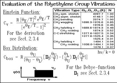
The next step in the analysis is to find an approximation for the spectrum of skeletal vibrations since, as mentioned above, the lowest skeletal vibrations are not well enough known, and often even the higher skeletal vibrations have not been established. To obtain the heat capacity due to the skeletal vibrations from the experimental data, the contributions of the group vibrations must be subtracted from Cv. A table of the group vibration frequencies for polyethylene can be derived from the normal mode analysis [22] in Fig. 2.47 and listed in Fig. 2.49. If such a table is not available for the given polymer, results for the same group in other polymers or small-molecule model compounds can be used as an approximation. The computations for the heat capacity contributions arising from the group vibrations are also illustrated in Fig. 2.49. The narrow frequency ranges seen in Fig. 2.47 are treated as

__________________________________________________________________

Fig. 2.49

single Einstein functions, the wider distributions are broken into single frequencies and box distributions as, for example, for the C C-stretching modes. The lower frequency limit of the box distribution is given by L, the upper one by U. The equation for the box distribution can easily be derived from two adjusted onedimensional Debye functions as shown in the figure.

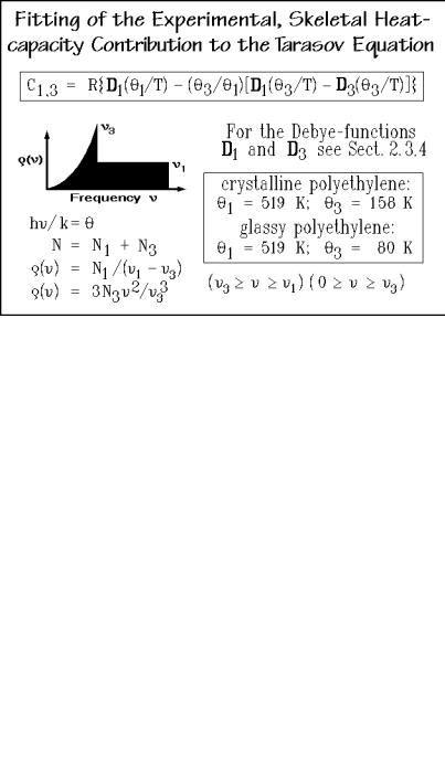
The next step in the ATHAS analysis is to assess the skeletal heat capacity. The skeletal vibrations are coupled in such a way that their distributions stretch toward zero frequency where the acoustical vibrations of 20–20,000 Hz can be found. In the lowest-frequency region one must, in addition, consider that the vibrations couple intermolecularly because the wavelengths of the vibrations become larger than the molecular anisotropy caused by the chain structure. As a result, the detailed molecular arrangement is of little consequence at these lowest frequencies. A threedimensional Debye function, derived for an isotropic solid as shown in Figs. 2.37 and 38 should apply in this frequency region. To approximate the skeletal vibrations of linear macromolecules, one should thus start out at low frequency with a threedimensional Debye function and then switch to a one-dimensional Debye function.

Such an approach was suggested by Tarasov and is illustrated in Fig. 2.50. The skeletal vibration frequencies are separated into two groups, the intermolecular group between zero and 3, characterized by a three-dimensional -temperature, 3, and an intramolecular group between 3 and 1, characterized by a one-dimensional - temperature, 1, as expected for one-dimensional vibrators. The boxed Tarasov equation shows the needed computation. By assuming the number of vibrators in the intermolecular part is N× 3/ 1, one has reduced the adjustable parameters in the equation from three (N3, 3, and 1) to only two ( 3 and 1). The Tarasov equation is then fitted to the experimental skeletal heat capacities at low temperatures to get3, and at higher temperatures to get 1. Computer programs for fitting are available,