

Thermal Analysis of Polymeric Materials
.pdf46 1 Atoms, Small, and Large Molecules
__________________________________________________________________
by 24 static chains to define a fixed volume. Next, a predetermined amount of kinetic energy is distributed randomly among the 3700 mobile CH2-groups to raise the temperature to 80 K. After only few picoseconds mechanical and thermal equilibrium is approached and the atomic motion can be observed.
Figure 1.47 illustrates the initial state and two snapshots of the inner seven chains of a simulated crystal, 0.2 ps apart. Only the lower parts of the chains are drawn to better show the details. The x, y, and z axes of the projection correspond to the initial
Fig. 1.47
a-, b-, and c-axes of the unit cell which is described in Chap. 5. All chains exhibit skeletal vibrations. It will be shown that these vibrations contribute much of the lowtemperature heat capacity. Transverse deviations from the planar zig-zag chains are seen in most chains as soon as the simulation is initiated (marked at the top of the center figure). The wave-motion can be followed and is seen to travel up and down the chains (compare to the right figure). The second chain from the left displays a strong torsional oscillation, visible by the change in the appearance of the projection of the zig-zag chain. Finally, a check of the lengths of the chains reveals longitudinal vibrations. All possible skeletal vibrations can thus be identified in Fig. 1.47. Their frequencies range up to about 1.8×10¹³ Hz, a value derived from normal mode calculations which are discussed when analyzing heat capacities in Chap. 2 (see Fig. 2.7).
Figure 1.48 contains a block diagram of the distribution of the rotation angles at higher temperatures. Oscillations of small amplitude represent the overwhelming part of the torsional vibrations. A small amount of large-amplitude deviations is found at an angle that is slightly smaller than the expected gauche conformations at 60 and 240°. (Note that the convention chosen for is different from that of Figs. 1.36 and 37 by 180°, trans = 180°). The intermediate, eclipsed conformations

1.3 Chain Statistics of Macromolecules |
47 |
__________________________________________________________________
Fig. 1.48
are found only rarely. A detailed discussion of the gauche conformations which represent defects in polyethylene crystals, and their relation to crystal properties, will be given in Sect. 5.3.4.
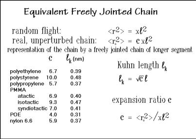
1.3.9 Equivalent Freely Jointed Chain
To represent real, unperturbed polymer molecules with the much simpler randomflight formalism, Kuhn1 introduced the equivalent, freely jointed chain by defining a longer segment that gives an identical mean square end-to-end distance with the same number of links x as a random flight of segments of length would give [16]. The new, longer segment is called the Kuhn length, k. Results for some flexible molecules are given in Fig. 1.49. The equations permit an easy correlation between the two definitions, the Kuhn length, and an expansion ratio c. All listed polymers would be characterized as flexible. The values of k should be compared to the C C bond length of 0.154 nm.
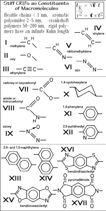
1.3.10 Stiff Chain Macromolecules
Four types of macromolecules of largely different Kuhn length are listed at the top of Fig. 1.50. Below this list, the repeating units which lead to molecules of different stiffness are drawn. The repeating units I and II can be found in most of the flexible molecules. Their inclusion in a polymer backbone introduces the angle in the structure which, together with a rather unhindered rotation about the connecting
1 W. Kuhn (1899–1963) Professor at the University of Basel, Switzerland.
48 1 Atoms, Small, and Large Molecules
__________________________________________________________________
Fig. 1.49
bonds, produces the flexibility. Some inorganic molecules, such as Si and Se, also can produce rather flexible macromolecules. Inclusion of occasional small, more rigid groups do not significantly increase the Kuhn length, such as is indicated by the aliphatic polyesters and amides (see the data for nylon 6.6 in Fig. 1.49).
The stiffest molecules are reached when the bond-angle between the backbone bonds is 180 degrees, such as in linking groups like III, XI, XII, and XV to XVII. For molecules such as polyparaphenylene, the Kuhn length approaches infinity and the molecules belong to the rigid macromolecules which are classified in Fig. 1.6 and in Fig. 1.7 a list representative is given.
To design molecules of different stiffness, one can couple the building blocks of Fig. 1.50. To produce flexibility, short and bent segments are required and steric hindrance due to bulky side groups must be small. Increasing the steric hindrance on rotation, lengthening the straight segments, and increasing the bond angle to 180°, and proper placement of crank-shaft-like segments (as IV IX, XIII, and XIV) are the tools to tailor-make stiffer molecules. The 1,4-cyclohexylene repeating unit (X) has an internal mobility, known from the easy interchange between its chair and boat conformations.
To appreciate the multiplicity of polymer molecules and their conformations, one should review the following points: 1. The many ways the repeating units can be linked together. 2. The uncountable number of molar mass distributions and conformations each single sample can have. 3. The large numbers of different degrees of stiffness that can be produced, ranging from the most flexible polymer to linear, rigid macromolecules. Knowledge about these topics permits the design of new materials of optimum properties and leads to the understanding of the behavior of already known polymeric materials, the elusive goal of every modern material scientist.
1.3 Chain Statistics of Macromolecules |
49 |
__________________________________________________________________
Fig. 1.50
50 1 Atoms, Small, and Large Molecules
__________________________________________________________________
1.4 Size and Shape Measurement
1.4.1 Introduction
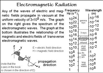
In this last section of Chap. 1, experimental methods are discussed to obtain data for the characterization of macromolecular sizes and shapes. The scattering of light is selected as the major method. It provides three pieces of information, the molecular size, shape, and the interaction parameters of the macromolecule with solvents [17,18]. The scattering of light is thus a versatile technique. Furthermore, its theory describes also the scattering of other electromagnetic radiation, as is summarized in Fig. 1.51, and even the scattering of neutrons and electrons, as described in Fig. 1.72,
Fig. 1.51
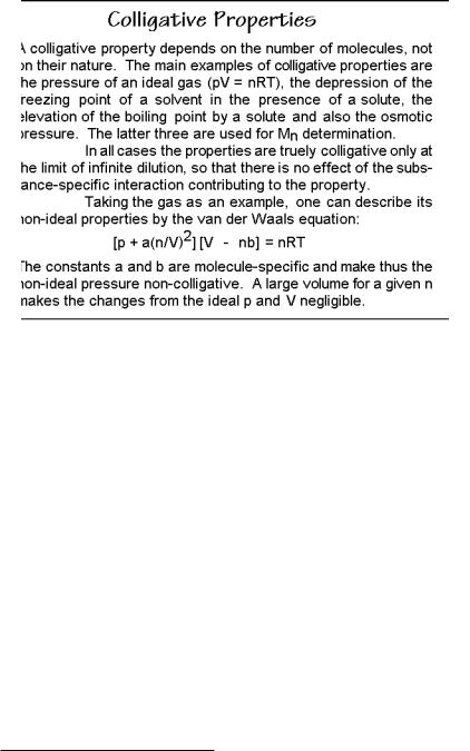
below. Light scattering is only one of the twelve techniques mentioned in this section. Details are also given for the colligative properties, explained in Fig. 4.52 (freezing temperature, boiling temperatures, and osmotic pressure), the semiempirical techniques of membrane osmometry and size-exclusion chromatography, and also the solution viscometry. Five additional characterizations are mentioned at the end of the chapter (Sect. 1.4.7).
1.4.2 Light Scattering
Light is one of the basic experiences of man. Ancient speculations about its nature abound. Pythagoras, the Greek philosopher and mathematician of the 6th century BC, suggested that light travels in straight lines from the eye to the object and that the sensation of sight arises from the touch of the light rays on the object. This feeling with light is still anchored in our language. The verb to see is used in the active
1.4 Size and Shape Measurement |
51 |
__________________________________________________________________
Fig. 1.52
voice. With present-day knowledge one must reverse the direction of the flow of information from the object to the eyes, i.e., to see should be passive.
The physical nature of light rays was a puzzle for many years. In the 17th and 18th centuries, theories about the wave nature (Huygens 1596 1687) and particle character (Newton 1643 1727) were proposed. By the 19th century the wave concept dominated, based on the precise descriptions of electromagnetic waves by Maxwell (1831 1879). Only in the 20th century could both concepts be joined by the discovery of matter waves (de Broglie, 1924). In the 19th century Richter developed as a first step of quantification the turbidity equation: = (1/ ) ln (Io/I), where is the length traveled by light of initial intensity Io, and I is the reduced intensity due to turbidity . The theory of light scattering as accepted today was then created by Lord Rayleigh1 [19].
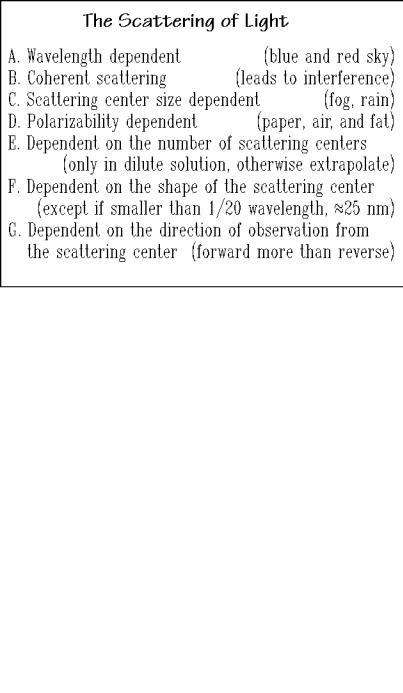
In our daily life, the scattering of light explains a number of well-known effects, listed in Fig. 1.53. The observations A D are basic experiences. The wavelength dependence of the scattering of light ( 4) causes the often brilliant colors of the sky, ranging from the blue sky overhead to the red evening sky. The coherence of scattered light permits interference of light scattered from different parts of objects as explained in Fig. 1.54. The size of the scattering centers can be linked to the observed intensities. Small water droplets in fog scatter so much that vision is completely obscured, while a much larger amount of water concentrated in bigger rain drops hinders vision only little. The dependency of light scattering on difference in polarizability, , which is proportional to the square of the refractive index, n,
1 John William Strutt (1842–1919), in 1873 he succeeded to the title Third Baron Rayleigh of Terling Place; professor at Cambridge University, England, Nobel Prize for Physics, 1904.
52 1 Atoms, Small, and Large Molecules
__________________________________________________________________
Fig. 1.53
leads, for example, to the loss of scattering of light on adding grease to paper, making it translucent. Paper appears white because of the large difference in n between the cellulosic fibers of paper (n = 1.55) and air located in the spaces between the fibers with n 1.00. Replacement of air with fat (n = 1.46) makes this difference in n disappear. Somewhat more advanced observation techniques are needed to detect the effects from E to G. The interference of light originating from different particles
Fig. 1.54
1.4 Size and Shape Measurement |
53 |
__________________________________________________________________
leads to a decrease in scattering intensity from concentrated solutions. As soon as the particles of the scattering centers are larger than about 25 nm in different directions, the shape of the scattering centers becomes of importance and leads to different scattering intensities. Finally, the direction of observation of scattered light is of importance. All these factors must be explained by the theory of light scattering. If some of these phenomena are not fully familiar to you, check the popular composition by Heller, who taught at the University of Detroit in the 1960s, which has been reprinted as Appendix 2.
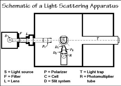
The experimental set-up for the scattering of light is shown in Fig. 1.55. The primary beam of light enters from the left and traverses the polymer solution contained in the cell C. The scattered light with an intensity i at an angle to the
Fig. 1.55
incident light beam is measured with the photomultiplier tube R. Modern equipment uses laser light and employs computer analysis for the data treatment.
The experimentation requires also a sensitive differential refractometer to separately evaluate the change of the refractive index of the polymer solution with concentration. Producing clean solutions is a paramount experimental condition, since all foreign particles scatter light and reduce the accuracy of the measurement. Furthermore, stray light must be kept from the photomultiplier, accomplished by a light-proof enclosure and a light trap T to eliminate the residual light from the incident beam. The angular dependence is measured by rotating R to different positions. In the shown instrument, the angles of 45, 90, and 135° are preset and match the cell walls.
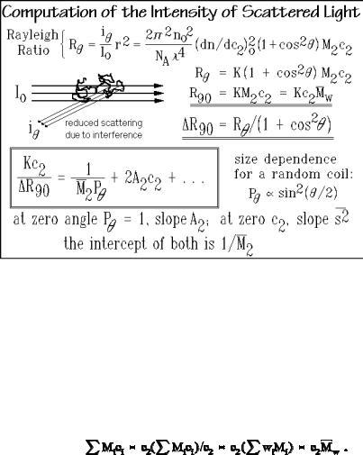
Figure 1.56 illustrates the computation of the molar mass average, M2 from the light-scattering results. The Rayleigh ratio R is the ratio of the scattered light intensity in direction to the primary light intensity Io at a distance r from the scat-
54 1 Atoms, Small, and Large Molecules
__________________________________________________________________
Fig. 1.56
tering center. Because of the somewhat lengthy nature of the detailed derivation of the Rayleigh ratio, it is given as Appendix 3. Figure 1.56 links the experimental Rayleigh ratio to the wavelength, , of the light used, the refractive index of the solvent, no, the change of n with polymer concentration c2, the molar mass of the polymer M2, the polymer concentration c2 (in Mg m 3), and the angle of scattering, expressed as .
The Rayleigh ratio simplifies on collecting all constants, the independently measured refractive index, and its change with concentration into a constant, K. Even simpler is the result when measuring at = 90° when 1 + cos2 = 1. If more species of molecules with molar masses Mi and concentrations ci are present, the massaverage is to be used. It is derived as follows from Sect. 1.2:
The equations just presented have two shortcomings. They apply only under the conditions of a very dilute solution, so that the scattered light from different particles does not interfere (see Fig. 1.54), and the scattering particles themselves are less than 25 nm in size, so that the light scattered from different parts of the same molecule does not interfere either.
Both of the shortcomings caused by interference can be corrected by appropriate extrapolations. The first extrapolation is carried to zero concentration c2, the second to zero scattering angle, . Understanding these two extrapolations does permit the extraction of two additional characterization parameters of the polymer from the same light-scattering experiment. The first extrapolation yields the interaction parameter between polymer and solvent. The second extrapolation yields an estimate of the molecular shape.
1.4 Size and Shape Measurement |
55 |
__________________________________________________________________
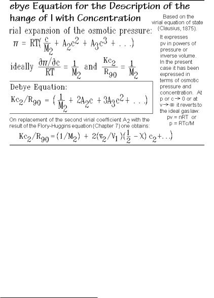
The extrapolation of the light-scattering data as a function of concentration was first given by Debye1 as shown in Fig. 1.57. One can write the equation for Kc2/R90 as an expansion in powers of c2 by noting the similarity of the concentration
Fig. 1.57
dependence of the osmotic pressure in a non-ideal solution to that of the inverse Raleigh ratio. The result is also listed in Fig. 1.56 for the case of terminating the expansion with the second term. The coefficient A2 (second virial coefficient) can be obtained from the slope of a plot of Kc2/ R90 vs. c2. The bottom equation in Fig. 1.57 shows the changes necessary if one wants to describe polymer solution with the Flory-Huggins equation, discussed in Chap. 7.
The dependence of light-scattering data on the angle is also mentioned in Fig. 1.53. It is accounted for by the factor P that corrects for the interference of the scattered light from different parts of the same molecule. The proportionality of factor P to the angle is derived by summing of all contributions to the scattered light from the macromolecule. A detailed expression for the change of P with angle is given in Fig. 1.58 for several shapes. It can be derived from statistical considerations, leading to results as shown in the figure for the random coil, discussed in Sect. 1.3.
Separating the angular dependence found earlier for small particles by dividing the Rayleigh ratio by (1 + cos2 ), one obtains R90, which is still -dependent because of the intermolecular interference. As expected, there is no reduction in the
1 Peter JW Debye (1884–1966), born in Maastricht, The Netherlands. Taught physics at the Universities of Zürich, Utrecht, Göttingen, and Leipzig. Director of the Kaiser Wilhelm Institute for Theoretical Physics, Berlin, from 1935, and from 1940 Professor of Chemistry at Cornell University, Ithaca, NY. Nobel Prize for Chemistry in 1936 (work on atomic dipoles).