Метод Т-матриц / Wriedt-superellipsoids-PartPartSystCharact-2002

Abstract

Light scattering by non-axisymmetric particles is commonly needed in particle characterization and other fields. After much work devoted to volume discretization methods to compute scattering by such particles, there is renewed interest in the T-matrix method. We extended the null-field method with discrete sources for

T-matrix computation and implemented the superellipsoid shape using an implicit equation. Additionally, a triangular surface patch model of a realistically shaped particle can be used for scattering computations. In this paper some exemplary results of scattering by nonaxisymmetric particles are presented.

1 Introduction

In optical particle characterization, light scattering computations are commonly needed. They help in the design of new instruments or in the investigation of the influence of various particle characteristics, such as shape, refractive index, composition or surface roughness, on a specific optical particle sizing instrument. Various other parameters of the instrument can also be easily investigated using light scattering simulations. For instance, the effect of the wavelength of the incident laser beam, the effect of particle trajectory through a measurement volume or the influence of the Gaussian intensity distribution of a laser beam can be computed. There is continuous interest in particle shape characterization. This would help to tell apart, e.g., non-spherical particles from spherical particles or fibrous particles from other particles. To develop new instruments for particle shape recognition, of course light scattering theories and corresponding computer programs for non-spherical particles are needed. The different methods available in this field have recently been reviewed by Wriedt [1] and Jones [2]. For this introduction, the various theories can be divided into volume-based and surface-based

*Dr.-Ing. T. Wriedt, Institut f¸r Werkstofftechnik, Badgasteiner Str. 3, 28359 Bremen (Germany).

E-mail: thw@iwt.uni-bremen.de

theories. Well known volume discretization methods are the various integral equation methods such as the discrete dipole approximation (DDA) [3], the volume integral equation method (VIEM) [4] and the differential equation method finite difference time domain method (FDTD)[5, 6]. Because the whole volume of a scatterer is discretized, the computer time is rather long. Nevertheless, these methods have been applied to compute scattering by non-spherical particles in optical particle sizing and in other fields. Scattering by cubic crystals has been studied using DDA [3] and scattering by ice crystals has been investigated using FDTD [5].

Since only the surface of a scattering body is discretized, the computer demand should be lower with surfacebased methods, but these methods have not yet been much applied to the computation of scattering by arbitrarily shaped particles.

The T-matrix method (also called the null field method or extended boundary condition method) is the best known of these methods because fast computer codes are easily available [7, 8], but it is mainly applied to scattering by axisymmetric scatterers. The T-matrix method was originally developed by Waterman [9 ± 11]. The T-matrix is based on expansion of all fields ± the incident, transmitted and the scattered field ± into a series of spherical vector wavefunctions.

A crucial advantage of the null-field method is that the transition matrix or the T-matrix relating the scattered

and the incident field coefficients can be computed in an easy manner. The T-matrix depends only on the incident wavelength and particle shape, its refractive index and its relation to the coordinate system. Thus, knowing a T- matrix, scattering by a rotated particle, a system of particles, a particle on a plane surface, in an incident Gaussian laser beam and orientation averaged scattering can easily be computed.

Taking into account the general properties of the T- matrix, Mishchenko elaborated an efficient analytical method for computing orientationally averaged light scattering characteristics for ensembles of non-spherical particles [12]. On the other hand, the T-matrix for a single scatterer can be used successfully for solving a large class of boundary-value problems in electromagnetic scattering theory. In this context, we mention the analysis of multiple scattering problems [13, 14] and the simulation of light scattering by layered or composite objects [15 ± 17] and by particles deposited on a surface [18].

However, for particles with extreme geometries or particles with appreciable concavities, the single spherical coordinate based null-field method fails to converge. A number of modifications to the conventional null-field method have been suggested for improving the numerical stability. These techniques include formal modifications of the single spherical coordinate-based null-field method [19 ± 21], different choices of basis functions [22, 23] and the application of the spheroidal coordinate formalism [24, 25]. One of these formal modifications is the null-field method with discrete sources [26 ± 28]. Essentially, this method entails the use of a number of elementary sources for approximating the surface current densities. The discrete sources are placed on a certain support in an additional region with respect to the region where the solution is required. Unknown discrete sources amplitudes which produce the surface densities are computed by using the null-field condition of the total electric field inside the particle surface. With this method, computation of the scattering by highly elongated or flat scatterers such as fibres and plates [29] and layered particles [30] is easily possible and the standard T-matrix can also be computed [31] for post-processing such as cluster scattering or orientation averaging.

Some brief comments on the history of the T-matrix method for non-axisymmetric particles may be of interest. Early scattering computations for non-axisym- metric scatterers using the T-matrix method were done by Barber [32] and by Schneider and Peden [33], both presenting results for ellipsoids.

The null field method with discrete sources has also been extended for the computation of scattering by nonaxisymmetric scatterers [34] and the method has been fully tested by comparison with other methods [35], giving results for cubes.

A 3D variant of the T-matrix method has also been developed by Laitinen and Lumme [36] and by Kahnert et al. [37], both presenting scattering results for rounded cubes, and another one by Havemann and Baran [38], giving results for hexagonal ice crystals.

To describe the scattering body using smooth functions, Laitinen and Lumme [36] expanded the surface of the scattering cube into a series of spherical harmonics. The problem with this method is that artificial roughness is introduced in addition to rounding of the edges of the cube. In optical particle characterization, mainly computations of scattering by some basic particle shapes have been investigated, such as spheres, spheroids, ellipsoids, cubes and finite cylinders. Because there is a lack of tools to describe particle shape, in the following the superellipsoid is proposed to generate various interesting particle shapes and it is integrated into the null field method with discrete sources.

The structure of the paper is arranged as follows. First the superellipsoid particle shape is described; next the null field method with discrete sources is briefly introduced and finally some examples of computational results are presented.

2 Superellipsoid

The superellipsoid represents a family of three-dimen- sional shapes as the product of two superquadratic curves [40]. This shape is well known in computer graphics and it can be used to model a wide range of shapes such as spheres, ellipsoids and cylinders and especially cubes and cylinders with rounded edges[39]. The superellipsoid is implemented in various computer programs used in computer graphics such as POV-Ray, so that a visualization of its form is easily available. The superellipsoid or superquadratic ellipsoid might be considered a generalization of the ellipsoid, and its implicit form is given by the equation

We use the same nomenclature as in POV-Ray. n is the north-south roundedness, e is the east-west roundedness and the bounds in x, y, z are given by the parameters a, b, c. The parametric form of the equation may also be useful in the construction of an object. The parametric equation of the superellipsoid is given by

If n and e are not equal to 1, the angles of course no longer correspond to the coordinates of the spherical coordinate system. A problem would arise in the equation if cos!t" or sin!t" was negative. In this case a negative number could have a fractional exponent, which is an illegal operation. Therefore, the interpretation, that !t"p has the same sign as t and the same magnitude as t p is adopted by using the following operator:

To produce only convex shapes, the values for n and e would be bounded: 0 n e 2. To prevent numerical overflow and difficulties with singularities, it is advisable to use a further bound: 0 1 n e 1 9. The variety of particle shapes, which can be modelled using the superellipsoid equation is plotted in Figure 1.

The variables n and e are varied between 0.2 and 2.0, whereas the bounds a, b and c are kept constant. One can see that a variety of shapes including a sphere, rounded cube, circular or rectangular cylinder, octahedra up to even some star-shaped objects can be generated.

The volume of a superellipsoid can be computed from [40]

The term B!x y" is the beta function, which is related to the gamma function:

The volume of some exemplary superellipsoids is given in Table 1.

Table 1: Volume of some exemplary superellipsoids.

V 8abc 7.657abc 6.482abc 5.538abc 4.189abc 1.333abc

Fig. 1: Examples of superellipsoids with parameters: e $ 0 2 1 0 1 0 0 2 2 0 and n $ 0 2 0 2 1 0 1 0 2 0. (left to right). a $ b $ c $ 1 0.

Fig. 2: Form of rounded cubes used for computation e $ n $ 0 2

For the exemplary computation, in the following section the rounded cube shapes depicted in Figure 2 will be used. The parameters n and e are 0.2, 0.5 and 0.7 such that cubes with different roundedness result.

3 Null-field Method with Discrete Sources

In this section we outline the basics of the null-field method with discrete sources[28]. Let us consider a threedimensional space D consisting of the union of a closed surface S its interior Di and its exterior Ds We denote by kt the wavenumber in the domain Dt where kt $ k t t

k $ c and t $ s i.

The transmission boundary-value problem can be formulated as follows. Let E0 H0 be an entire solution to the Maxwell equations representing an incident electromagnetic field. Find the vector fields, Es Hs C1!Ds" C!Ds" and Ei Hi C1!Di" C!Di" satisfying the Max-

n Hi n Hs $ n H0

on S In addition, the scattered field Es Hs must satisfy the Silver-M¸ller radiation condition uniformly for all directions x x It is known that the transmission boun- dary-value problem posseses a unique solution[41].

For solving the transmission boundary-value problem in the framework of the null-field method with discrete sources, the scattering object is replaced by a set of surface current densities e and h, so that in the exterior domain the sources and fields are exactly the same as those existing in the original scattering problem. The entire analysis can conveniently be broken down into the following three steps:

(I) A set of integral equations for the surface current densities e and h is derived for a variety of discrete

2n # 1 !n m " Dmn $ 4n!n # 1" !n # m "

1mn3 !kx" $ M1m3m#l!k!x zne3"" x R3 zne3 n$11mn3 !kx" $ N1m3m#l!k!x zne3"" x R3 zne3 n$1

!11"

We recall that a system i i$1 is called a Schauder basis of a Banach space X if any element u X can be uniquely represented as u $ i$1 i i where the convergence of the series is in the norm of X It is noted that in the case of localized vector spherical functions the notion of Schauder basis is closely connected with the Rayleigh hypothesis. This hypothesis says that the series

representation of the scattered field in terms of radiating localized vector spherical functions, which uniformly converges outside the circumscribing sphere, also converges on S

(III) Once the surface current densities have been determined, the scattered field outside the circumscribing sphere is obtained by using the representation theorem. We obtain the series representation

Here, is a complex index incorporating m and n, i.e.

$ ! m n"

3.1 T-matrix Computation

Now, for deriving the T-matrix let us assume that the incident field can be expressed inside a finite region containing S as a series of regular vector spherical functions

Then, using Eqs. (8) ± (18) we see that the relation between the scattered and the incident field coefficients is linear and is given by a transition matrix T as follows:

and A , B and A0 are block matrices written in general as

with X standing for A B and A0 Explicit expressions for the elements of these matrices are given in the Appendix. It is noted that the exact infinite T-matrix is independent of the expansion systems used on S. However, the approximate truncated matrix, computed according to

does contain such a dependence.

Energy characteristics in the far field are computed from the far-field pattern ENs0 for a unit amplitude incident electric field for p- or s-polarization. The angle-depend- ent intensity function plotted in the simulation section is the normalized differential scattering cross-section (DSCS):

To compute numerically orientation-averaged scattering, three integrals with respect to the three Euler

angles have to be computed. Thus the value of interest f ! " is integrated over all directions and polarization of the incident plane wave. The numerical procedure used to do this is based an a stepwise procedure:

The triple integral is converted to three summations. The angle is digitized for N steps in the range !0 2 ", angleis digitized for N steps in the range !0 ", and angle is digitized for N steps in the range !0 2 "

4 Mesh Generation

Implicit surfaces are commonly used for modelling purposes in numerous scientific applications, including CAD system and computer graphics. Therefore, there are various interests in constructing a polyhedral representation of implicit surfaces [42]. In our case, the representation in a triangular patch model should allow first a correct calculation of surface integrals and second a graphical visualization of the particle. Different methods are available to create a geometric surface mesh.

To generate the superellipsoid shape for our light scattering simulations we use the HyperFun software

tool [43, 44] which is a program supporting high-level language functional representations in computer graphics. Function representation is a generalization of traditional implicit surfaces and constructive solid geometry which allows the construction of complex shapes such as isosurfaces of real-valued functions composed of functionally defined primitives and operations [45]. The HyperFun polygonizer used for surface mesh generation generates VRML output of a triangular patch model. HyperFun generates a sufficiently regular mesh which, although intended for computer graphics, is very well suited for our application, as we found.

An example of gridding is shown with the rounded cubes given in Figure 2. In these examples the dimensions are a $ b $ c $ 0 3 m and the numbers of triangular patches are 1448, 1448, 1400.

In the standard method to compute surface integrals, the parametric equation is used and therefore an equivalent integral in planar coordinates has to be evaluated. Hence, partial derivatives of x, y, z with respect to the parametrization (in our case parameters ) are needed, which may not be available analytically. If the partial derivatives are not available, a numerical method via finite differences may be used.

We use an alternative approach based on a modified centroid quadrature that does not use the partial derivatives. This modified centroid quadrature has been proposed and investigated by Georg and Tauch [46]. The surface integrals to be computed are approximated by

i

S

where, vi 1 vi 2 vi 3 are the vertices spanning a triangle and point vi c denotes the centre of mass of the triangle %vi 1 vi 2 vi 3& given by

Thus, the integral over each triangle is approximated by multiplying the value of the integrand at the centroid by the triangle area.

5 Numerical Simulations

5.1 Program Validation

The computer program based on the DSM theory was checked using various internal checks such as computing scattering by a shifted particle and comparing the result with scattering by the original particle.

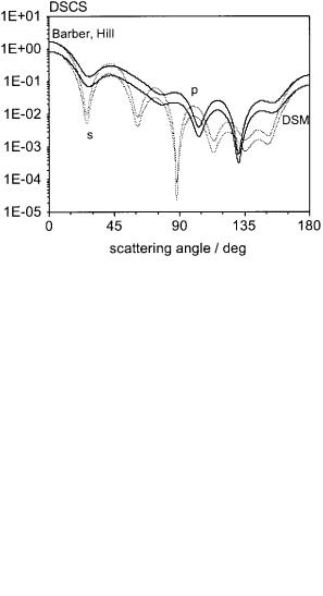
Next, the program was validated by comparing it with other programs. We used the T-Matrix programs t1 included with the book by Barber and Hill [7]. The first result is for a spheroid with dimensions of a $ b $ 500 nm and c $ 700 nm Practically no difference was found, as can be seen by the normalized DSCS for p- and s-polarization plotted in Figure 3. The T-Matrix result is shifted with respect to the DSM result because Barber and Hill apply a different normalization in the differential scattering cross section (DSCS) computed. To check the routine for orientation averaging, the program t5 of Barber and Hill [7] is used to compute a reference result of the orientation averaged DSCS for the same spheroid. The results of both computations are plotted in Figure 4 and there is perfect agreement between the

Fig. 4: Orientation-averaged differential scattering cross-section of spheroid a $ b $ 500 nm c $ 700 nm, 10725 faces, 1000 orientations, Nmax $ 16 Mmax $ 15 M $ 1 5 $ 628 31 nm

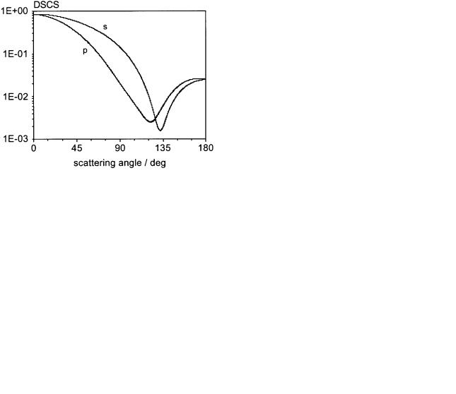
Fig. 5: Differential scattering cross-section of ellipsoid a $ 150 b $ 200 c $ 300 nm 11656 faces, 64 64, M $ 1 5, $ 628 31 nm pol $ 45

results computed by the DSM program and the t5 program.

As another example of program validation, scattering by an ellipsoid with dimensions a $ 150 b $ 200 and c $ 300 nm is presented in Figure 5. The comparative result of the DSCS was computed with another implementation of the same theory [34]. As can be seen, there is perfect agreement between the two sets of results.

To present a final example of program validation for nonaxisymmetric particles, the 3D-Multiple Multipole Program (MMP) of Hafner and Bomholt [47] was used for computation of a scattering result of a rounded cube for comparison with. This method is based on an expansion of the internal and the scattered field into so-called multipoles. A generalized point matching method is used to fulfil the boundary conditions on the surface of the scattering particle and to compute the coefficients of the expansion functions. In the example given we used spherical vector wavefunctions for field expansion. The FORTRAN code is available with the MMP book and this code was modified such that a triangular surface patch model of the scattering particle could be read into the program to be used for the point matching procedure. As mirror symmetry can be accounted for in the MMP program, only an eighth of the surface of the rounded cube has to be used for triangulation into a triangular surface patch model. In the example presented, this surface was covered by 1435 faces. The rounded cube was generated by the superellipsoid equation with the parameters e $ n $ 0 2 and a $ b $ c $ 1 0 m. The computational results of the differential scattering crosssection are plotted in Figures 6 and 7. Apart from some different normalization of the DSCS there is almost perfect agreement between the MMP and DSM results.

Fig. 6: Differential scattering cross-section (p-polarization) of rounded cube with parameters e $ n $ 0 2 a $ b $ c $ 1000 nm,

Nmax $ 20 Mmax $ 18 M $ 1 5 $ 628 31 nm, DSM: 14648 faces; MMP 1/8 of cube with 1435 faces.

Fig. 7: Differential scattering cross-section (s-polarization) of rounded cube with parameters e $ n $ 0 2 a $ b $ c $ 1000 nm

Nmax $ 20 Mmax $ 18 M $ 1 5 $ 628 31 nm DSM: 14648 faces; MMP 1/8 of cube with 1435 faces.

5.2 Convergence

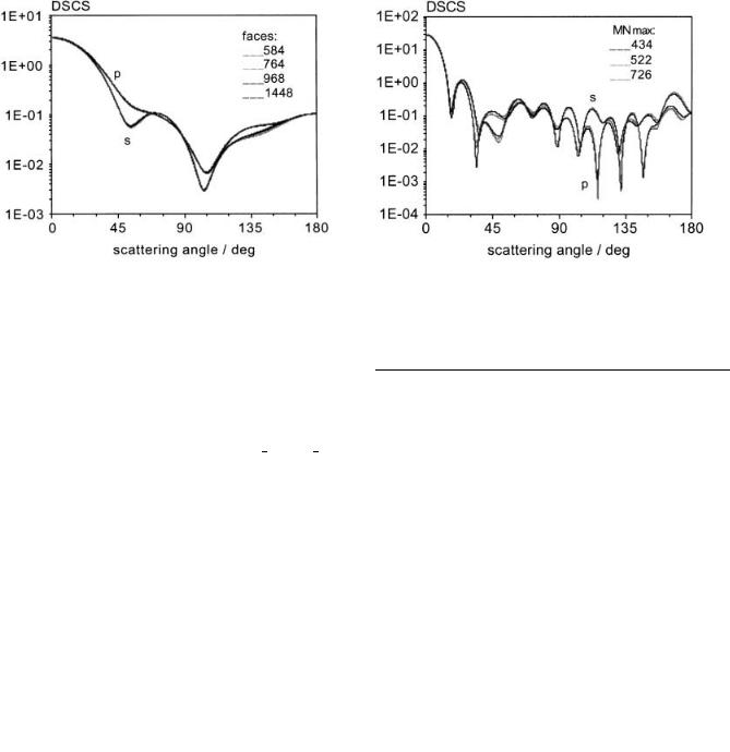
A profound convergence test is an important step in program testing. Two kinds of convergence checks have to be made: (a) versus the number of triangular faces of the particles, corresponding to the number of integration elements and, (b) versus the number of localized spherical vector wavefunctions used for field expansion. Figure 8 shows an exemplary result for a convergence test versus the number of integration elements (faces) for a rounded cube with parameters a $ 300 nm n $ e $ 0 2 and refractive index M $ 1 5. By comparing the curves it can be seen that convergence is easily reached and from further investigation we conclude that convergence

Fig. 8: DSCS computed for convergence test versus number of integration points (faces) for a cube. a $ b $ c $ 300 nm, n $ e $ 0 2, Nmax $ 10 Mmax $ 7 M $ 1 5 $ 628 31 nm

Fig. 9: DSCS computed for convergence test versus number of expansion functions MNmax for a cube a $ b $ c $ 1000 nm n $ e $ 0 5, 14648 faces, M $ 1 5 $ 628 31 nm

versus the number of integration elements seems to be mainly uncritical and can easily be achieved. Of more importance is a convergence check versus the number of expansion functions. This number depends on the

maximum value of the indices n and m (Nmax and Mmax) of the spherical vector wavefunctions M and N . This

number of expansion functions MNmax is given by

Table 2: Number of expansion functions.

This corresponds to a size of the transition matrix given by T!2MNmax 2MNmax" Various convergence checks were applied to test the program for different shapes of scatterers. An exemplary result of such a convergence test is given in Figure 9, where the differential scattering cross-section is plotted for a cube. The values of the

parameters Nmax and Mmax used in the simulation and the resulting corresponding number of expansion functions

MNmax are summarized in Table 2.

5.2.1 Scattering by Rounded Cube

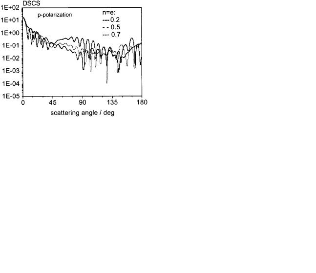
In this section, some sample results of single scattering by the superellipsoids pictured in Figure 2 are presented. Figures 10 and 11 give the differential scattering crosssections of a cube with dimensions a $ b $ c $ 1 5 m and different values of the two roundedness parameters. The first figure gives p-polarization and the second s- polarization.

Scattering by even larger rounded cubes is plotted in Figures 12 and 13, which give the differential scattering cross-section of a cube with dimensions and different values of the two roundedness parameters. The influence

Fig. 10: Differential scattering cross-section (p-polarization) of

of roundedness is especially seen in p-polarization at a scattering angle of 45 ± 90 .

Just a single exemplary scattering result for orientationaveraged scattering by a rounded cube with roundedness parameters e n $ 0 5 is given in Figure 14. The p-and s- polarization results almost become indistinguishable and

Fig. 11: Differential scattering cross-section (s-polarization) of rounded cube with different values of e and n a $ b $ c $ 1500 nm Nmax $ 30 Mmax $ 28, 33464 faces, M $1.5, $ 628 31 nm.

Fig. 12: Differential scattering cross-section (p-polarization) of rounded cube with different values of e and n,

a $ b $ c $ 2000 nm Nmax $ 39 Mmax $ 38, 76220 faces, M $ 1.5,$628 31 nm.

Fig. 13: Differential scattering cross-section (s-polarization) of rounded cube with different values of e and n a $ b $ c $ 2000 nm Nmax $ 39 Mmax $ 38, 76220 faces, M $1.5, $ 628 31 nm.

Fig. 14: Orientation averaged differential scattering cross-sec-

the angular variation in the DSCS is much smoother than that for the same particle in a fixed orientation.

5.2.2 Scattering by Realistically Shaped Particles

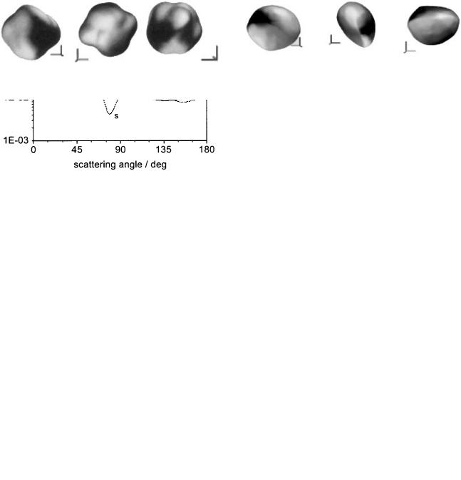
To demonstrate that scattering by an arbitrarily shaped particle is also possible with the program developed, the shape of asteroid KY26 was used. Its shape is available as a triangular surface patch model in the wavefront format on the Internet [48]. There are 4092 faces in the data file and the dimensions of the 0.030 km asteroid were scaled down by a factor of 100 m/km such that a particle with a range of 2.92 m in x, 2.64 m in y and 2.77 m in z resulted. Three different views of this KY26-shaped

particle are given in Figure 15. The number of triangular faces was increased to 16368 using a one-to-four triangular subdivision scheme. In Figure 16 the differential scattering cross-section is plotted. As orientation, the orientation given in the original data file was used with z being the direction of the incident plane wave. In Figure 17 the orientation-averaged differential scattering cross-section is given. It can be seen that the angular variation in the DSCS is smoother than that computed for the same particle in a fixed orientation.

To demonstrate that scattering from realistically shaped particles can be computed, a number of photographs of a pebble from different views were used to reconstruct a realistic particle shape. Similarly, electron micrography

Fig. 16: Differential scattering cross-section of KY26-shaped particle, Nmax $ 10 Mmax $ 7, 4092 faces, M $ 1 5, $ 628 31 nm

Fig. 19: Oriention-averaged differential scattering cross-section of ™real∫ shaped particle, 1728 orientations, Nmax $ 20 Mmax $ 17, 28032 faces, M $ 1 50, $ 628.31 nm.

Fig. 17: Oriention-averaged differencial scattering cross-section of KY26-shaped particle, 1000 orientations, Nmax $ 10 Mmax $ 7, 4092 faces, M $ 1 5, $ 628 31 nm

from different views of a small particle could be used to reconstruct its 3D shape. The geometry of the pebble was reconstructed from an image sequence of apparent contour profiles from 20 different viewpoints taken by an electronic camera [49].

Three views of the reconstructed realistically shaped particle are shown in Figure 18. The dimensions of the particle were scaled such that its size in x is 2.176 m in y

is 1.585 m and in z is 1.856 m. The shape of the particle was triangulated with 27745 faces. In Figure 19 the orientation-averaged differential scattering cross-sec- tion of this particle is plotted.

To generate an arbitrarily shaped particle with a different amount of surface roughness, the DOS program PovRockGen [50] was used. The dimensions of the particles generated are such that its overall size in x is 2.026 m, in y is 2.026 m and in z is 1.969 m. The parameters for generating the smooth particle are depth $ 4 and smoothness $ 2.0 and the parameters for generating the rough particle are depth $ 4 and smoothness $ 1.5. Originally 5120 surface triangles were generated. These were increased to 20480 by a one-to-four triangular subdivision scheme.

The two different kinds of particle shapes generated and used for scattering computations are shown in Figure 20 and the orientation-averaged computation results are plotted in Figure 21. With the smooth particle, oscillations in the scattering diagram are more pronounced. With the rougher particle, the amount of cross-polar- ization is, of course, increased.