The Equipment items are represented by dots, and you can see that there the Equipment items are located in the Chemical Plant area. The Buildings are represented by dark green/brown backwards diagonal pattern on the GIS and GIS Legend. The location data for a hazardous event is defined on the Equipment item, rather than on the Study or the Scenario.

The Display Order tab of the Legend for the GIS Input View controls the order in which the different

“layers” of information are displayed in the view. The Equipment layer is at the top, which means that the dots that represent the Equipment items will always be visible.

The Raster Image layers are always at the bottom so they appear in the background behind all of the other input data. In the illustration the Southpoint_OS image layer is above the Southpoint_Aerial image layer. If you swap these two image layers by dragging the Southpoint_OS to the bottom, the aerial photograph image will be displayed instead of the map image. You can also right click items in the legend and choose Display On or Display Off to show and hide items respectively.

The Risk tab section

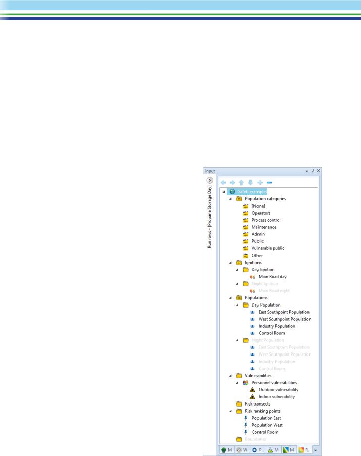
You use the Risk tab to define data that are specific to the risk calculations.

Categories

The program is supplied with a default list of Categories for Populations, with a different display style defined for each Category. Each Population is assigned to a Category, and the Category determines the style that will be used when displaying the Population in a GIS View.

The Category is also used in the risk results, where some forms of results provide an analysis according to the populations assigned to each Category.

Ignitions

The ignition sources are used in modelling the location and probability of delayed ignition, and the input data for each ignition includes the probability that it will ignite a flammable cloud. You can define ignition sources on the GIS View as points, straight lines, polylines, rectangular areas and polygon areas.

The distribution and strength of ignition sources typically varies according to the time of day, and the examples file reflects this, with separate folders of ignitions for day and night. The Day and Night Run Rows have different sets of ignitions selected, and the Night ignitions are shown as greyed out because the active Run Row is a Day row.

Populations

The risk modelling calculates fatalities for each population, and also considers populations as a potential cause of delayed ignition. The input data for each population includes the

proportion of people indoors and out of doors. You can define populations on the GIS View as points and as areas, and you can also use the Data source option in the Data tab of the Ribbon bar to import population shapes and population data from an external GIS database.