The Risk Supertabs

The Risk Supertabs appear in a separate pane inside the main window; this pane is normally located along the left side of the window. There are four tabs in this pane, arranged in an order from left to right that reflects the main stages in the process of performing a risk analysis.

The first Risk Supertab is the Input Supertab, which contains a separate panel called the Study Tree. The Study Tree covers all of the aspects of the input data for the consequence and risk calculations, with the different aspects of the data organised in separate tab sections. For example, the Models tab covers the

definition of hazardous Scenarios, and the Weather tab covers the definition of representative weather conditions for modelling. The different tabs of the Study Tree are described in the next section.

The next two Risk Supertabs are the Run Row Grid Supertab and the Combinations Supertab, which cover different aspects of the definition of the Run Rows that specify different combinations of aspects of the input data. In Safeti, a Run Row is a combination of input data from across the other tab sections, and you can use different Run Rows to calculate the risk for alternative scenarios (e.g. for day conditions and for night conditions), and then to combine or to compare the risks. The concept of a Run Row should become clearer after you have seen the setup of the input data in the Study Tree, and when you see the method for defining a Run Row in a later section of the tutorial.

The last Risk Supertab is the Results Supertab, which gives you a quick way of viewing risk results.

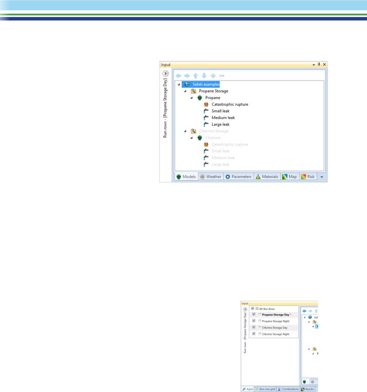
The other feature of the Risk Supertabs is the Run Row Selector, which is a special pane that is normally “collapsed” along the left side of the

Input Supertab, where it appears as a line of vertical text with a circular Hide/Show button at the top. If you click on the button or on the text, the Run Row Selector pane will become expanded, and will push the Study Tree pane to the right, as shown in the illustration. The Run Row Selector pane lists all of the Run Rows that are defined in the workspace, and you can see that four Run Rows are defined in the Safeti examples file: there are separate rows defined for day conditions and for night conditions for the propane and for the chlorine releases.

You use the Run Row Selector to choose one of the Run Rows as the active Run Row, and also to select the Run Rows to be calculated and to perform the calculations. The selection for the active run row affects various aspects of how the input data are displayed and checked. The Row selected as the active Run Row is shown by an orange asterisk *, and when the Run Row Selector is collapsed, the name of the active Run Row is displayed in the line of vertical text; in the Safeti examples file, the active Run Row is set to Propane Storage Day.