

3.Risk Contour Results
These results present the geographical distribution of the risk of exceeding vulnerability criteria, in the forms of contours for a given level of risk displayed in a GIS View. The different types of risk contour results allow you to compare different aspects of the risk levels.
For a full description of each form of risk results, you should refer to the online Help. Enter “Risk Results” in the Index tab of the Help window to view a summary list of all of the available types of risk results, with links to the details of each type.
Viewing the risk results
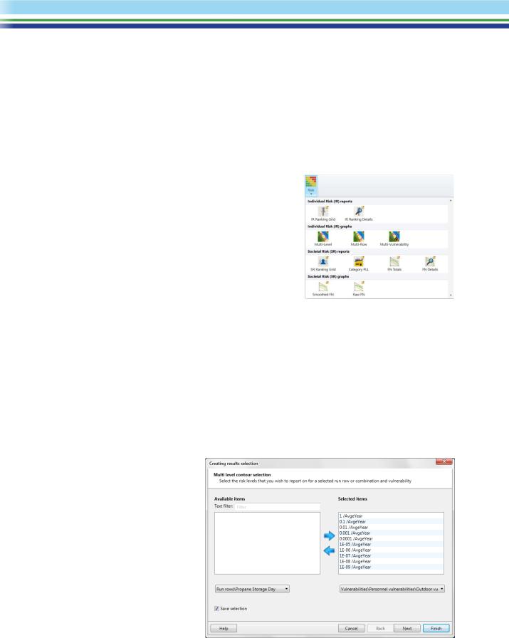
To view a particular form of risk results, either select it from the right-click menu for a node in the Run Row Selector pane as describe aboved, or select it from the Risk gallery in the Home tab of the Ribbon Bar, as shown.
The Risk gallery is always available, no matter which tab of the Study Tree or Supertabs you are working in. You do not have to have the Run Row Selector pane open in order to view risk results using the Risk gallery.
Whenever you select the option to view a form of risk results, a Results Selection Wizard dialog will appear. This dialog is similar to the dialog that appears when you view a form of consequence results, though the details of the options in the dialog can be very different, depending on the type of risk results that you want to view. The other main difference from the selection dialog for viewing consequence results is that the selection dialog for risk results gives you the choice to save the definition of the combination of options that you have selected. You can then use that saved combination at any time and viewing the risk results more quickly.
This tutorial describes the process of viewing two forms of risk contours and one of the grid-based forms of societal risk results, and of saving and using a Results Selection.
Multi-Level risk contours for day and night combined
Select the Multi-Level option for risk contours from the Risk gallery. This type of plot allows you to select multiple risk contours levels for plotting, and will display a separate contour for each level.
When the selection dialog opens, it will have some selections already made as shown in the illustration. These selections are discussed below.
The risk levels to be modelled in the risk contour calculations are defined in the Risk Preferences dialog, which you open by clicking on the Preferences option in the
Settings tab of the Ribbon Bar. When the dialog opens, all of these defined levels will be selected and in the Selected items list at the right of the dialog. If you do not want to plot a particular level, you can click on it and then click on the left arrow to move it to the Available items list.
| SAFETI | April 2018 | www.dnvgl.com/software |
Page 22 |
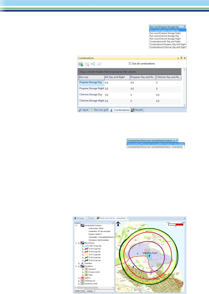
The dropdown field below the Available items field lists all of the Run Rows and also all of the Combinations, as shown.
The results for a given Combination are the combination of the results for the different Run Rows, using the weighting factor for each Run Row that are defined for that Combination in the Combinations Supertab.
The Safeti examples file has three Combinations, defined as shown. The All: Day and Night Combination includes
the propane and the chlorine results, with a factor of 0.4 for the Day rows and a factor of 0.6 for the Night rows, meaning that daytime conditions are assumed to apply for 40% of the year. The other two Combinations use the same weighting factors for Day and Night, but cover only propane or only chlorine.
When the selection dialog opens, the Propane Storage Day Row will be selected because it is the first in the list, but you should change the selection to Combinations\All: Day and Night.
The dropdown field below the Selected items field lists all of the sets of vulnerability criteria that are defined under the Vulnerabilities
folder in the Risk tab section of the Study Tree. The risk calculations for each Run Row produce separate risk contour results for each set of vulnerabilities, and you must choose which of these sets of results you want to view. When the selection dialog open, the Outdoor vulnerability set will be selected because it is the first in the list, and you can leave it with this selection.
The other field in the dialog is the Save selection checkbox at the bottom left. This field is always checked when the dialog first open. If you leave the field checked, the program will add an entry for the current combination of options to the Results Supertab. For this contour plot, you should leave the box checked.
The Next button will take you to the last screen in the Wizard dialog, which allows you to give a name and description for the saved selection. For this contour plot, you can click on Finish in the first screen of the Wizard dialog.
After you click on Finish a GIS Risk Results View will open as shown. You can see that the highest risk level over the offsite populated areas to the south of the plant is slightly higher than 1x10⁻⁵/AvgeYear as the contours for 1x10⁻⁵ stop just reach the residential area and the town. The highest risk onsite is around the propane vessel, near the centre of the plant, but there is a visible
| SAFETI | April 2018 | www.dnvgl.com/software |
Page 23 |
contribution from the chlorine vessel, further to the west.
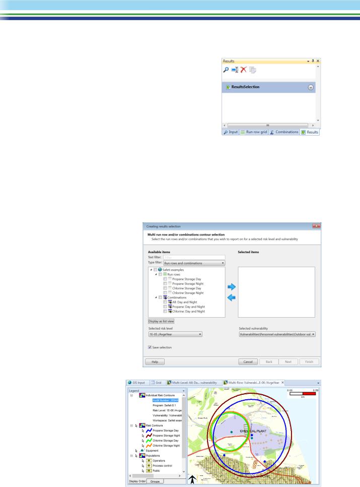
If you move to the Results Supertab, you will see that it contains one entry, called ResultsSelection. This is the default name that will be used for any new Results Selection if you do not supply a name in the final screen of the Wizard dialog. You can rename a saved Results Selection at any time, and also delete or duplicate one.
Rename this Results Selection All Combination. You will use it later for viewing societal risk results for the same Combination.
Multi-Row contours for a risk level of 1x10⁻⁶/AvgeYear
The Multi-Row contour plot allows you to plot separate contours for different Run Rows, for a selected risk level. For this plot you will set the risk level as 1x10⁻⁶/AvgeYear, since this is the highest contour that crosses the populated areas in the combined plot.
Most of the selections for this plot will be different than those for the previous plot, so you would not save time by using the saved Selection. Instead, select the Multi-Row option for risk contours from the Risk gallery to create a new Selection.
When the Wizard dialog first opens, the list of Available items will include all Run Rows and all Combinations as shown. Check the box by the Run rows node and click on the right arrow to move all of the Run Rows to the Selected items list.
For a Multi-Row plot, the dropdown field under the Available items field lists all of the risk levels available. 1x10⁻⁶/AvgeYear is the default setting in this situation, so you can leave the field with this setting.
You can also leave the selection of vulnerability criteria with the default setting of Outdoor, and leave Save selection checked.
When you click on Finish, the Multi-
Row plot will open in a second GIS
Risk Results View, as shown.
| SAFETI | April 2018 | www.dnvgl.com/software |
Page 24 |
Category PLL societal risk results for day and night combined
The Category PLL results give the societal risk in terms of the Potential Loss of Life. The PLL for a particular outcome is the number of fatalities multiplied by the frequency. The Category PLL results show the contribution to the total PLL from different Scenarios and types of hazardous effect, and also the contribution from fatalities in different Population Categories.
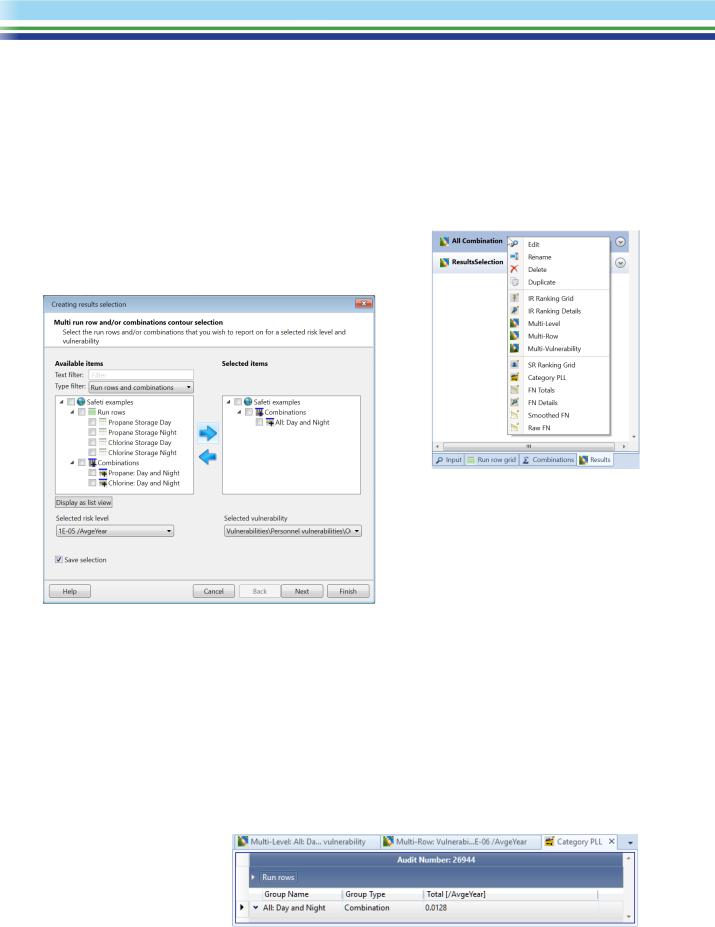
You will use the saved All Combination Selection in the Results Supertab to view the Category PLL results. If you right-click on the Selection, you will see a list of the available types of risk results, as in the Risk gallery.
When you select Category PLL from the list, the Wizard dialog for the Category PLL results will appear as shown below.
The form of the dialog for the Category PLL results is different from the form of the dialog for the MultiLevel Risk Contours, but the relevant aspects of the selection have been applied, and the All: Day and Night Combination has been selected. You can leave this selection unchanged.
If you leave the Save selection box checked when viewing results from a saved Selection, the program will not create a separate saved Selection, but will update the definition of the saved Selection with the selections that you make in the current dialog. If you want to keep the original definition of the saved Selection, you must uncheck the box. For this tutorial, you can leave the box checked.
The Wizard dialog for Category PLL also has several additional screens that allow you to select only specific Scenarios or specific types of hazardous effect, but for this tutorial you can click on Finish in the first screen to include all Scenarios and types of effect.
The Category PLL View will open in a separate tab next to the contour plots, as shown. When it first opens it will be fully collapsed, and will be showing the total value for the PLL, calculated as a weighted average across all Run Rows.
| SAFETI | April 2018 | www.dnvgl.com/software |
Page 25 |
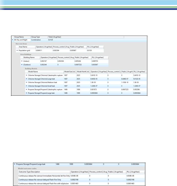
This type of results view is organised in several levels, and you can drill down level by level to analyse the contributions to the risk. In the illustration below, the report has been expanded to the fourth level, which shows the individual Scenarios (or “Models”).
In the Category PLL view, the second level is Areas; if you do not have a license for the 3D Explosion modelling, this will only ever show one row, with the name “Population grid” as shown. For this level and all levels below, there are columns that show the PLL for populations in different Categories in addition to the total PLL, and you can see that almost all of the PLL is in the Industrial Category.
The third level is Buildings, which shows the contribution from outdoor and indoor populations. You can see that the Indoor PLL is about five times the Outdoor PLL.
The fourth level is Models, which lists the individual Scenarios. Here you can see that the propane releases dominate the risk.
You can expand under a Scenario down to the fifth level, which is the type of hazardous effects (known as the “outcome codes”), as shown below for the large Propane Leak. You can see that the risk is dominated by the flash fire and explosion from delayed ignition of the gas cloud, with only a small contribution from the jet fire from immediate ignition.
You have now seen the main features of Safeti. When you are ready you should proceed to Chapter 2, which takes you through the stages in setting up your own analysis.
| SAFETI | April 2018 | www.dnvgl.com/software |
Page 26 |