Part I: Getting Started with Excel

Moving around a Worksheet

This section describes various ways to navigate through the cells in a worksheet. Every worksheet consists of rows (numbered 1 through 1,048,576) and columns (labeled A through XFD). After column Z comes column AA, which is followed by AB, AC, and so on. After column AZ comes BA, BB, and so on. After column ZZ is AAA, AAB, and so on.

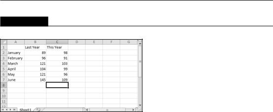
The intersection of a row and a column is a single cell. At any given time, one cell is the active cell. You can identify the active cell by its darker border, as shown in Figure 1.2. Its address (its column letter and row number) appears in the Name box. Depending on the technique that you use to navigate through a workbook, you may or may not change the active cell when you navigate.

Notice that the row and column headings of the active cell appear in different colors to make it easier to identify the row and column of the active cell.

8

Chapter 1: Introducing Excel

FIGURE 1.2

The active cell is the cell with the dark border — in this case, cell C8.

Navigating with your keyboard

Not surprisingly, you can use the standard navigational keys on your keyboard to move around a worksheet. These keys work just as you’d expect: The down arrow moves the active cell down one row, the right arrow moves it one column to the right, and so on. PgUp and PgDn move the active cell up or down one full window. (The actual number of rows moved depends on the number of rows displayed in the window.)

Tip

You can use the keyboard to scroll through the worksheet without changing the active cell by turning on Scroll Lock, which is useful if you need to view another area of your worksheet and then quickly return to your original location. Just press Scroll Lock and use the navigation keys to scroll through the worksheet. When you want to return to the original position (the active cell), press Ctrl+Backspace. Then, press Scroll Lock again to turn it off. When Scroll Lock is turned on, Excel displays Scroll Lock in the status bar at the bottom of the window. n

The Num Lock key on your keyboard controls how the keys on the numeric keypad behave. When Num Lock is on, the keys on your numeric keypad generate numbers. Many keyboards have a separate set of navigation (arrow) keys located to the left of the numeric keypad. The state of the Num Lock key doesn’t affect these keys.

Table 1.2 summarizes all the worksheet movement keys available in Excel.

9

Part I: Getting Started with Excel

TABLE 1.2

Navigating with your mouse

To change the active cell by using the mouse, click another cell; it becomes the active cell. If the cell that you want to activate isn’t visible in the workbook window, you can use the scrollbars to scroll the window in any direction. To scroll one cell, click either of the arrows on the scrollbar.

To scroll by a complete screen, click either side of the scrollbar’s scroll box. You also can drag the scroll box for faster scrolling.

Tip

If your mouse has a wheel, you can use the mouse wheel to scroll vertically. Also, if you click the wheel and move the mouse in any direction, the worksheet scrolls automatically in that direction. The more you move the mouse, the faster the scrolling. n

Press Ctrl while you use the mouse wheel to zoom the worksheet. If you prefer to use the mouse wheel to zoom the worksheet without pressing Ctrl, choose File Options and select the Advanced section. Place a check mark next to the Zoom on Roll with Intellimouse check box.

Using the scrollbars or scrolling with your mouse doesn’t change the active cell. It simply scrolls the worksheet. To change the active cell, you must click a new cell after scrolling.

10

Chapter 1: Introducing Excel

Introducing the Ribbon

The most dramatic change introduced in Office 2007 was the new user interface. In most Office 2007 applications, traditional menus and toolbars were replaced with the Ribbon. In Office 2010, all applications use the Ribbon interface. In addition, the Ribbon can be customized in Office 2010 (see Chapter 23).

Ribbon tabs

The commands available in the Ribbon vary, depending upon which tab is selected. The Ribbon is arranged into groups of related commands. Here’s a quick overview of Excel’s tabs.

•Home: You’ll probably spend most of your time with the Home tab selected. This tab contains the basic Clipboard commands, formatting commands, style commands, commands to insert and delete rows or columns, plus an assortment of worksheet editing commands.

•Insert: Select this tab when you need to insert something in a worksheet — a table, a diagram, a chart, a symbol, and so on.

•Page Layout: This tab contains commands that affect the overall appearance of your worksheet, including some settings that deal with printing.

•Formulas: Use this tab to insert a formula, name a cell or a range, access the formula auditing tools, or control how Excel performs calculations.

•Data: Excel’s data-related commands are on this tab.

•Review: This tab contains tools to check spelling, translate words, add comments, or protect sheets.

•View: The View tab contains commands that control various aspects of how a sheet is viewed. Some commands on this tab are also available in the status bar.

•Developer: This tab isn’t visible by default. It contains commands that are useful for programmers. To display the Developer tab, choose File Options and then select Customize Ribbon. In the Customize the Ribbon section on the right, place a check mark next to Developer and then click OK.

•Add-Ins: This tab is visible only if you loaded an older workbook or add-in that customizes the menu or toolbars. Because menus and toolbars are no longer available in Excel 2010, these user interface customizations appear on the Add-Ins tab.

Note

Although the File button shares space with the tabs, it’s not actually a tab. Clicking the File button displays the new Back Stage view, where you perform actions with your documents. n

11

Part I: Getting Started with Excel

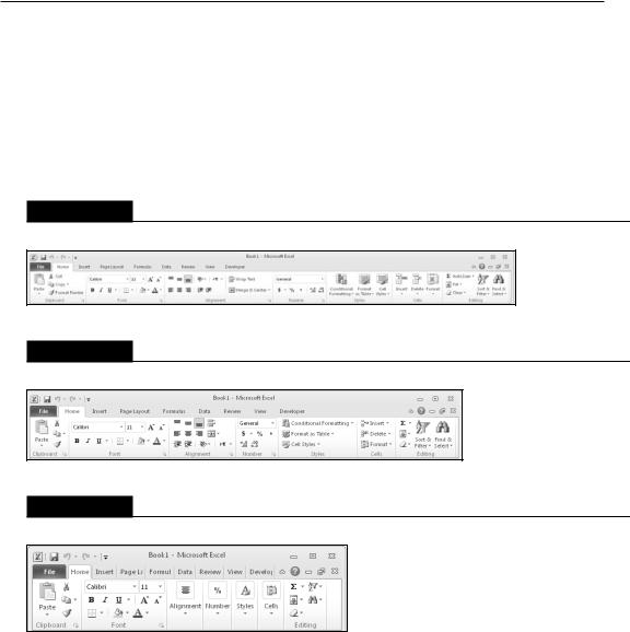
The appearance of the commands on the Ribbon varies, depending on the width of Excel window. When the window is too narrow to display everything, the commands adapt; some of them might seem to be missing, but the commands are still available. Figure 1.3 shows the Home tab of the Ribbon with all controls fully visible. Figure 1.4 shows the Ribbon when Excel’s window is made more narrow. Notice that some of the descriptive text is gone, but the icons remain. Figure 1.5 shows the extreme case when the window is made very narrow. Some groups display a single icon. However, if you click the icon, all the group commands are available to you.

FIGURE 1.3

The Home tab of the Ribbon.

FIGURE 1.4

The Home tab when Excel’s window is made narrower.

FIGURE 1.5

The Home tab when Excel’s window is made very narrow.

Tip

If you would like to hide the Ribbon to increase your worksheet view, just double-click any tab. The Ribbon goes away, and you can see about five additional rows of your worksheet. When you need to use the Ribbon again, just click a tab, and it comes back temporarily. To keep the Ribbon turned on, double-click a tab. You can also press Ctrl+F1 to toggle the Ribbon display on and off. The Minimize the Ribbon button (to the left of the Help button) provides yet another way to toggle the Ribbon. n

12

Chapter 1: Introducing Excel

Contextual tabs

In addition to the standard tabs, Excel 2010 also includes contextual tabs. Whenever an object (such as a chart, a table, or a SmartArt diagram) is selected, specific tools for working with that object are made available in the Ribbon.

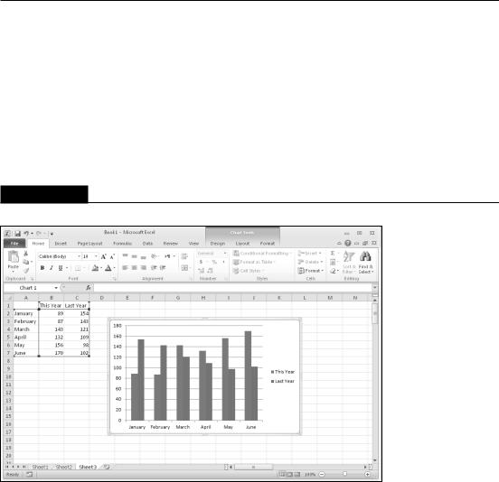
Figure 1.6 shows the contextual tab that appears when a chart is selected. In this case, it has three contextual tabs: Design, Layout, and Format. Notice that the contextual tabs contain a description (Chart Tools) in Excel’s title bar. When contextual tabs appear, you can, of course, continue to use all the other tabs.

FIGURE 1.6

When you select an object, contextual tabs contain tools for working with that object.

Types of commands on the Ribbon

When you hover your mouse pointer over a Ribbon command, you’ll see a pop-up box that contains the command’s name as well as a brief description. For the most part, the commands in the Ribbon work just as you would expect them to. You do encounter several different styles of commands on the Ribbon.

13

Part I: Getting Started with Excel

•Simple buttons: Click the button, and it does its thing. An example of a simple button is the Increase Font Size button in the Font group of the Home tab. Some buttons perform the action immediately; others display a dialog box so that you can enter additional information. Button controls may or may not be accompanied by a descriptive label.

•Toggle buttons: A toggle button is clickable and also conveys some type of information by displaying two different colors. An example is the Bold button in the Font group of the Home tab. If the active cell isn’t bold, the Bold button displays in its normal color. If the active cell is already bold, though, the Bold button displays a different background color. If you click this button, it toggles the Bold attribute for the selection.

•Simple drop-downs: If the Ribbon command has a small down arrow, the command is a drop-down. Click it, and additional commands appear below it. An example of a simple drop-down is the Conditional Formatting command in the Styles group of the Home tab. When you click this control, you see several options related to conditional formatting.

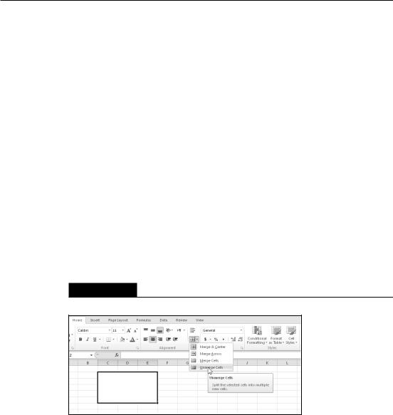
•Split buttons: A split button control combines a one-click button with a drop-down. If you click the button part, the command is executed. If you click the drop-down part (a down arrow), you choose from a list of related commands. You can identify a split button command because it displays in two colors when you hover the mouse over it. An example of a split button is the Merge & Center command in the Alignment group of the Home tab (see Figure 1.7). Clicking the left part of this control merges and centers text in the selected cells. If you click the arrow part of the control (on the right), you get a list of commands related to merging cells.

FIGURE 1.7

The Merge & Center command is a split button control.

•Check boxes: A check box control turns something on or off. An example is the Gridlines control in the Show group of the View tab. When the Gridlines check box is checked, the sheet displays gridlines. When the control isn’t checked, the sheet gridlines don’t appear.

•Spinners: Excel’s Ribbon has only one spinner control: the Scale To Fit group of the Page Layout tab. Click the top part of the spinner to increase the value; click the bottom part of the spinner to decrease the value.

14

Chapter 1: Introducing Excel

Some of the Ribbon groups contain a small icon on the right side, known as a dialog box launcher. For example, if you examine the Home Alignment group, you see this icon (see Figure 1.8). Click it, and Excel displays the Format Cells dialog box, with the Alignment tab preselected. The dialog launchers generally provide options that aren’t available in the Ribbon.

FIGURE 1.8

Some Ribbon groups contain a small icon on the right side, known as a dialog box launcher.

Accessing the Ribbon by using your keyboard

At first glance, you may think that the Ribbon is completely mouse-centric. After all, none of the commands have the traditional underline letter to indicate the Alt+keystrokes. But in fact, the Ribbon is very keyboard friendly. The trick is to press the Alt key to display the pop-up keytips. Each Ribbon control has a letter (or series of letters) that you type to issue the command.

Tip

You don’t need to hold down the Alt key while you type keytip letters. n

Figure 1.9 shows how the Home tab looks after I press the Alt key to display the keytips. If you press one of the keytips, the screen then displays more keytips. For example, to use the keyboard to align the cell contents to the left, press Alt, followed by H (for Home) and then AL (for Align Left). Nobody will memorize all these keys, but if you’re a keyboard fan (like me), it takes just a few times before you memorize the keystrokes required for commands that you use frequently.

After you press Alt, you can also use the leftand right-arrow keys to scroll through the tabs. When you reach the proper tab, press the down arrow to enter the Ribbon. Then use left and right arrow keys to scroll through the Ribbon commands. When you reach the command you need, press Enter to execute it. This method isn’t as efficient as using the keytips, but it’s a quick way to take a look at the commands available.

15