


1232 |
CHAPTER 17. WIRELESS INSTRUMENTATION |
17.1.7Link budget graph
Many of the concepts previously explored may be represented in a single graph13, showing RF signal strength as a function of physical position within the RF link (from transmitter to receiver). The horizontal axis of this graph represents the position along the link path from transmitter to receiver, while the vertical axis represents RF signal strength in dBm:
|
|
|
Transmitter |
Transmitter |
Transmitter |
|
Transmitting |
Path loss, |
Receiving |
Receiver |
Receiver |
Receiver |
||||||
|
|
|
output power |
arrestor |
cable |
|
antenna |
etc. |
antenna |
cable |
arrestor |
input power |
||||||
Regulatory limit |
|
|
|
|
|
|
|
|
|
|
|
|
|
|
|
|
|
|
|
|
|
|
|
EIRP |
|
|
|
|
|
|
|
|
|
||||
|
|
|
|
|
|
|
|
|
|
|
|
|
||||||
|
|
|
|
|
|
|
|
|
|
|
|
|
|
|
|
|
||
|
|
|
|
|
|
|
|
|
|
|
|
|
|
|
|
|
|
|
|
|
|
|
|
|
|
|
|
|
|
|
|
|
|
|
|
|
|
|
|
|
|
|
|
|
|
|
|
|
|
|
|
|
|
|
|
|
Signal power |
|
|
|
|
|
|
|
|
|
||
|
|
|
|
|
|
|
|
|
|||
|
|
|
|
|
|
|
|
|
|||
(dBm) |
|
|
|
|
|
|
|
|
|
||
|
|
|
|
|
|
|
Margin |
||||
|
|
|
|
|
|
|
|
|
|
||
Receiver |
|
|
|
|
|
|
|
|
|
||
|
|
|
|
|
|
|
|
|
|||
|
|
|
|
|
|
|
|
|
|||
sensitivity (Prx(min)) |
|
|
|
Minimum signal/noise ratio |
|||||||
|
|||||||||||
|
|
|
|
||||||||
|
|
|
|
|
|
|
|||||
|
|
|
|
|
|
|
|
|
|
|
|
Noise floor (Nf) |
|
|
|
Noise figure (Nrx) |
|||||||
|
|
|
|||||||||
|
|
|
|||||||||
|
|
|
|
|
|
|
|
|
|
|
|
|
|
|
|
|
|
|
|
|
|
||
|
|
|
|
|
|
|
|
|
|
|
|
|
|
|
|
Position in system |
|||||||
At the very bottom of this graph we see the noise floor, representing natural RF noise that is unavoidable. Above that we see the added noise figure and signal/noise ratios summing up to a higher line representing the receiver’s sensitivity, which is the minimum amount of signal power it must receive in order to reliably function.
Near the top of this graph we see a series of thicker line segments representing the various losses and gains within the system. Single-point losses such as lightning arrestors appear as vertical downward steps, while progressive losses such as cables and path loss appear as downward slopes. Single-point gains such as antennas appear as vertical upward steps. Note where EIRP appears on this graph: the amount of signal power at the transmitting antenna’s output, factoring in the antenna’s gain as well as any losses between the transmitter and the transmitting antenna. As previously mentioned, the Federal Communications Commission (FCC) sets regulatory limits for EIRP in the United States, because if only the transmitter’s output power were regulated, it would be possible to thwart that limit using high-gain antennas.
At the far right-hand end of the graph, we see the di erence between the receiver’s input signal power and the receiver’s sensitivity as a margin for the link budget. This margin must exist in order to grant the system tolerance to unexpected power losses such as those resulting from inclement weather, interference from objects within the link path, cable deterioration, coupling corrosion, increases in noise floor, etc.
13I am indebted to Eric McCollum, Kei Hao, Shankar V. Achanta, Jeremy Blair, and David Kechalo for presenting this form of diagram in a technical paper presented at the 45th annual Western Protective Relay Conference in Spokane, Washington in October of 2018. I do not know if these authors are responsible for the invention of this form of graph, but it was certainly the first time I encountered one like it, and it so clearly showed all the fundamental quantities of an RF link budget that I had to include something similar in my book!
17.1. RADIO SYSTEMS |
1233 |
17.1.8Fresnel zones
One of the many factors a ecting RF link power transfer from transmitter to receiver is the openness of the signal path between the transmitting and receiving antennas. As shown in the previous subsection, path loss is relatively simple to calculate given the assumption of totally empty space between the two antennas. With no obstacles in between, path loss is simply a consequence of wave dispersion (spreading). Unless we are calculating an RF link budget between two airplanes or two spacecraft, though, there really is no such thing as totally empty space between the transmitting and receiving antennas. Buildings, trees, vehicles, and even the ground are all objects potentially disrupting what would otherwise be completely open space between transmitter and receiver.
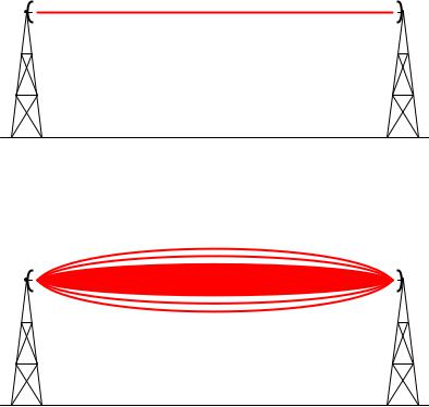
A common expression in microwave radio communication is line-of-sight, or LoS. The very wording of this phrase evokes an image of being able to see a straight path between transmitting and receiving antennas. Obviously, if one does not have a clear line-of-sight path between antennas, the signal path loss will definitely be more severe than through open space. However, a common error is in thinking that the mere existence of an unobstructed straight line between antennas is all that is needed for unhindered communication, when in fact nothing could be further from the truth:
Antenna |
False model of radio wave distribution |
Antenna |
line-of-sight
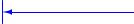
In fact, the free space necessary to convey energy in electromagnetic wave form takes on the form of football-shaped zones: the first one solid followed by annular (hollow) zones concentrically surrounding the first. These elliptical volumes are called Fresnel zones:
Fresnel zones
Antenna |
Antenna |
The precise shapes of these Fresnel zones are a function of wavelength and distance between antennas, not the size or configurations of the antennas themselves. In other words, you cannot change the Fresnel zone sizes or shapes by merely altering antenna types. This is because the
1234 |
CHAPTER 17. WIRELESS INSTRUMENTATION |
Fresnel zones do not actually map the distribution of electromagnetic fields, but rather map the free space we need to keep clear between antennas14.
If any object protrudes at all into any Fresnel zone, it diminishes the signal power communicated between the two antennas. In microwave communication (GHz frequency range), the inner-most Fresnel zone carries most of the power, and is therefore the most important from the perspective of interference. Keeping the inner-most Fresnel zone absolutely clear of interference is essential for maintaining ideal path-loss characteristics (equivalent to open-space). A common rule followed by microwave system designers is to try to maintain an inner Fresnel zone that is at least 60% free of obstruction.
In order to design a system with this goal in mind, we need to have some way of calculating the width of that Fresnel zone. Fortunately, this is easily done with the following formula:
r = r |
|
D |
|
|
nλd1d2 |
Where,
r = Radius of Fresnel zone at the point of interest
n = Fresnel zone number (an integer value, with 1 representing the first zone) d1 = Distance between one antenna and the point of interest
d2 = Distance between the other antenna and the point of interest D = Distance between both antennas
λ = Wavelength of transmitted RF field, in same physical unit as D, d1, and d2
Note: the units of measurement in this formula may be any unit of length, so long as they are all the same unit.
D
Antenna |
Antenna |
r

 d1
d1 
 d2
d2
14The physics of Fresnel zones is highly non-intuitive, rooted in the wave-nature of electromagnetic radiation. It should be plain to see, though, that Fresnel zones cannot describe the actual electromagnetic field pattern between two antennas, because we know waves tend to spread out over space while Fresnel zones converge at each end. Likewise, Fresnel zones vary in size according to the distance between two antennas which we know radiation field patterns do not. It is more accurate to think of Fresnel zones as keep-clear areas necessary for reliable communication between two or more antennas rather than actual field patterns.