3456

Issue № 4(32), 2016 ISSN 2075-0811

The discrepancy of strain is as follows

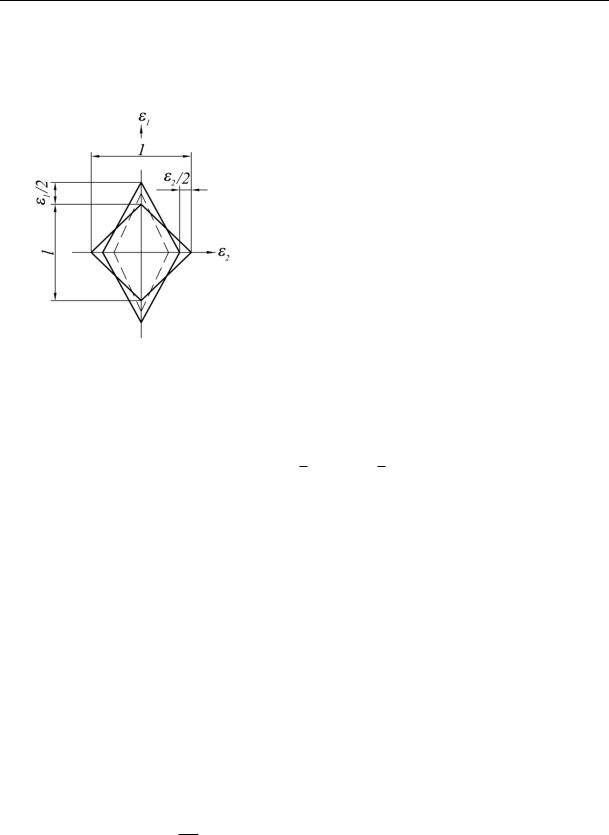
The deformations corresponding with the strains {σр} i consist of the elastic {εр} i and plastic {е} i parts. According to the Huke’s law, the coaxiality of σе1,2,3 and εе1,2,3, σр1,2,3 and εр1,2,3 in the space (or a plane) of the major strains, i.e. the major deformations.

Fig. 1. Graphic illustration for the iterative meth-

od of elastic solutions for the version of the meth-

od of initial strain

The graphic illustration of the above is a two-dimensional analogy which is a Prandtl diagram in Fig. 1. For a complex strain (stress-strain accompanied by changes in the shape) the general deformations include the linear (elastic) and plastic parts with the plastic component of deformations emerging as the yield point is achieved as specified in the design model of an object in question. The diagram ОЕ1Р1ЕiРi… depicts iteration of solving an elastic plastic task. The points Еi depict the connections between the strains and deformations {σе}i – {εе}i according to the Huke’s law and the points Рi the strains {σр}i determined depending on{σе}i.

In order to obtain the relations between{σе}i and {σр}I, let us introduce two known assumptions of the plastic flow theory.

1. Speed tensors of plastic deformations {е} and strains {σр} are coaxial. Therefore the vectors of the main strains σе1,2,3, σр1,2,3, of elastic εе1,2,3, εр1,2,3 and plastic е1,2,3 deformations are on the same axes and can be summed (subtracted) with no considerations of coaxiality thus

The equation (3) according to the scheme in Fig. 1 expresses the quality of the sum of the elastic and plastic deformations on the strains σр1,2,3, i and deformations εе1,2,3, i obtained in the

“elastic” solution of a task at the first stage of each (i-th) iteration step.

2. Vectors of plastic deformations are connected by some function F(σр) = 0 called “a plastic potential” and describing a plane (a curved or straight line) in the space of strains with the following ratio:

61

Scientific Herald of the Voronezh State University of Architecture and Civil Engineering. Construction and Architecture

where λ is a small positive scalar value; ekj , e1,2,3 are increases in the (speed) of plastic deformations along the coordinate axes (kj) or axes of major strains and deformations. Mathematically the ratio (4) means the vector of plastic deformations ekj , e1,2,3 is perpendicu-

lar to the plane of a plastic potential.

The function Fр(σр) = 0 describing the yield point or a limit strain can be used as a plastic potential at the points of the design area. In this case the law would be associated, which suggests that the equations be written generally (in the associated manner) describing the yield point and vector of plastic deformations.

There are functions F(σр) = 0 describing other (non-associated) yield laws but such equations are mostly analogues of the yield functions with the accuracy of constant coefficients.

Obtaining resolving equations. In the resistance of materials theory and technical guidelines for metal structures, foundations and geomaterials as yield (loading) functions Fр(σр) = 0 the Huber-Mises (energetical theory of strength), Mohr-Coulomb, Mises-Schleicher-Botkin equations are used. Equations providing the implementation of the method of elastic solutions and method of initial strain using the mathematical foundation of the method of finite elements to

meet the conditions of the above laws of plastic yield. 1. The Mohr-Coulomb law:

where φ, c are the strength characteristics of the foundation: the angle of the interior friction and specific cohesion; Λ* is a dilatancy parameter expressing the ratio of the volumetric deformation to changes in the shape for flat deformation.

The equation (6) describes a plastic potential of a non-associated yield law where Λ* substitutes sinφ in the yield equation (5). The plastic deformation of an elementary volume of the foundation for flat deformation is according to the scheme in Fig. 3 using the equation

where е1,2 are the plastic components of the major deformations; λ is a small scalar value equation to the angle of shift.

62

Issue № 4(32), 2016 ISSN 2075-0811

Fig. 2. Changes in the shape and dilatancy of an elementary volume of the foundation for plastic deformation:

1 are the original sizes;

2 is a shift for the constant volume (Λ* = 0);

3 is a change in the shape with the dilatancy (Λ* > 0)

The coefficient Λ* ≠ 0 makes the deformation based on equation (7) different from the flow in a constant volume where е1,2 = ±½λ and the areas inclined under the angle of 450 in relation to the axes of the major strains is as follows:

е /4 0, р /4 12 е1 – е2 12 .

In relation to the flat deformation conditions of foundations considering the yield point (5) using the pair of equations (3) the plastic potential equaiton (6) is as follows:

formation of changes in the shape with dilatancy. The right parts of the equations express relative deformations 1,2e 21G [(1 ) 1,2e e2,1 ] .

Unknown major strains σ1,2р must meet the yield point conditions (5).

Equations (9) and (5) make up an isolated system whose solution allows one to obtain the following links between σ1,2р and σ1,2е [3]:

63

Scientific Herald of the Voronezh State University of Architecture and Civil Engineering. Construction and Architecture

In the finite elements of “the failure region” Fе > 0.

Here as later on (for solutions of spatial tasks), the transition from “discrepancy of forces” Δσ1,2, I = σр1,2, I – σe1,2, i to the axial strains Δσх, i, Δσz, i, Δτxz, i is theoretically not challenging and needs no explanation.

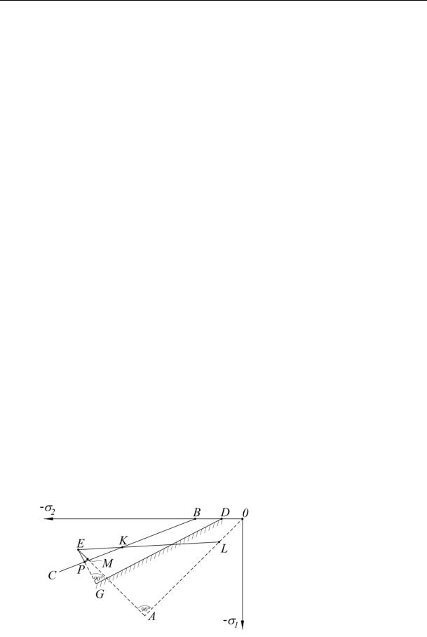
Fig. 3 presents the plane of the major strains σ1,2, the boundary straight line ВKРС depicts the Mohr-Coulomb Fp = 0, line DG — the plastic deformation F(σр1,2) according to equation (6), dotted line ОА — a hydrostatic axis. Let us look at the connection between the graphic forms of strains σ1,2p and σ1,2е. Let us assume that segment LE depicts changes in the stress strain at the point (elementary volume) of the design area after load application: the point L (σ1,2 = –р) corresponds to the initial (natural) pressure; point Е (σ1,2е) is the result of a linear solution of the task, the stress strain that it depicts is physically impossible.

Acurally as vector LE crosses boundary straight line ВС (point K), the stress strain takes on the plastic stage defined by the line ВKР. Point Р depicts strains σ1,2p according to (11). Projection of line ЕР onto axes σ1,2 depicts the difference between strains σ1,2р and σ1,2е:

ЕР Fе (1– 2 * ) / (1– 2 * sin ),

consisting of deviator ЕМ and hydrostatic МР parts:

ЕМ F е 1 – 2 / (1 – 2 * sin ), МР –F е * / (1 – 2 * sin ).

Fig. 3. Graphic representation of the connections between σp1,2 and σе1,2

on the plane of the major strains

64

2. The flow equation of Mises-Schleicher-Botkin for spatial stress strain is as follows:

where I1 is the first invariant of the stress tensor:

I1 1 2 3 ;

I2 is the second invariant of the stress deviator:

I2 1/ 6 1 – 2 2 2 – 3 2 3 – 1 2 ;

α and k are the strength characteristics of foundations similar to sinφ and с defined using the method of three-axial compression in accordance with the GOST (ГОСТ) 12248-2010; Λ is a dilatancy parameter for the conditions of spatial stress strain.

More specifically the ratios (4) and (3) for the conditions of the task at hand result in the following equations:

whereе l, m, n — 1, 2, 3; the other denominations remain unchanged.

The system of three equations (16) and equation (13) in relation to the unknown σ1,2,3р and λ are solved as described below.

The following ratio is the resutl of summing three equations (16):

Subsequent substraction of the second equation from the first, the third from the second, the first from the third, squaring of each obtained equation, summing of three new equations and division into 6 results in the following

or (after the extraction of the root from the left and right parts and simple transformations)

65

Scientific Herald of the Voronezh State University of Architecture and Civil Engineering. Construction and Architecture

Inserting (17), (18) into (13):

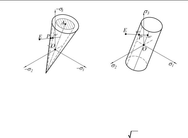
Fig. 4а shows graphic representations of the plastic potential (14) as a cone plane inserted into a cone describing the equation of Mises-Schleicher-Botkin (13). Line ЕР depicts the connections between the strains σе1,2,3 (point Е) and σр1,2,3 (point Р).

According to equation (15)

6J2p

where Jp1 and Jp2 is the first invariant of the tensor and the second invariant of the deviator of plastic deformations at the point of the design area.

3. The flow equation of Huber-Mises for spatial stress strain associated with the plastic potential

where σТ is the yield point or design resistance using the yield point. Equation (21) is a particular case of equations (13), (14) where

66

Issue № 4(32), 2016

Fig. 4. Graphic representation of the flow equation and connections between σp in spaces of major strains:

а) flow equations of Mises-Schleicher-Botkin (13), plastic potential (14); b) Huber-Mises (21)

Using these values in equations (17), (19), (20), we get

Fig. 4b shows graphic representation of equation (21) as a cylindrical space. Lines ЕР depict the connections of strains σp1,2,3 and σе1,2,3 in the space of major strains.

Example. Let us show the way the above ideas and calculation methods are implemented using the example of the solution of an axial symmetrical task to press a drilled pipe into a soil foundation [4]. The plastic component of the deformations of the design area is described by the Mises-Schleicher-Botkin (13) and the plastic potential (14). The frictional forces along the sides of the pipe are restricted with a specific resistance according to the designing standards.

A drilled pipe with the diameter of 1,7 m and the length of 26,8 m was made during the construction of a pipe foundation of a large bridge. As a well was drilled, three types of sand (φ = 28÷330) and four layers of clayous foundations (φ = 19÷270, с = 15÷54 kPа) were involved. The pipe was stopped at 1,6 m into dust sand (Е = 28 МPа, φ = 320) with the total capacity of 4,0 m. The bases were stiff loam (the capacity is 1,2 m, Е = 17 МPа, φ = 200,

с = 17 kPа), semi-solid clay (Е = 23 МPа, φ = 180, с = 40 kPа). The specific weights of the foundations was accepted to be γ = 19 kN/m3.

The pipe was tested in a design position. The load as high as 12,5 МN was reached and reduced due to the limit of the anchor system. The carrying capacity (yield resistance) of the pipe was not achieved.

67

Scientific Herald of the Voronezh State University of Architecture and Civil Engineering. Construction and Architecture

Through the course of the elastic plastic calculation modelling the test of the drilled pipe, the finite system calculation scheme with the radius of 10,2 m, the height of 37 m was used. The

load as high as 20 МN was reached.

б)

3×0,15

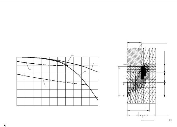
Fig. 5. Graphic representation of the exmple of the calculation of a drileld pipe with the diameter of 1,7 m:

а) diagrams of the dependences s = f (P): 1 — using the statistical test data;

2 — using the results of the elastic plastic calculation, 3 — elastic solution, 4, 5 — as the pipe is unloaded; b) areas of a specific stress strain: 1, 2, 3 — for the loads P respectively 15,0, 17,0 and 18,0 МN

The data in Fig. 5а show that there is a good agreement between the “subsidence-load” dependence in terms of the results of the elastic plastic solution and the static test. The design curve remained smooth till the end of the calculation. Fig. 5b shows the areas of a specific stress strain for three loads Р = 15,0, 17,0 and 18,0 МN. For the pressing force Р = 17,5 МN the area of a specific stress strain of the foundation under the lower end of the drilled pipe crossed the symmetrical axis of the design area and reached the height of 0,9 m (0,5 of the diameter of the pipe), the design subsidence was 80 mm (0,047 of the diameter of the pipe); the “elastic” component of the subsidence was 30 mm (37,5 % of the total subsidence), line 3 in Fig. 5а.

Conclusions

The resolving equations presented in the paper used for bilinear deformation diagrams with the conditions of plastic flow of Huber-Mises, Mohr-Coulomb, Mises-Schleicher-Botkin are the key element of iteration of the method of elastic solutions that allow the “initial strain” for

68

it to be implemented to be obtained. The suggested method of designing resolving equations can be employed in solving elastic plastic tasks with other equations describing a yield point, deformation at the plastic flow stage.

References

1.Gorodetskiy A. S., Zavoritskiy V. I., Lantukh-Lyashenko L. I., Rasskazov A. S. Avtomatizatsiya raschetov transportnykh sooruzheniy [Automation of calculations of transport facilities]. Moscow, Transport Publ., 1989.

232p.

2.Zenkevich O. Metod konechnykh elementov v tekhnike [Finite element method in engineering]. Moscow, Mir Publ., 1975, 375 p.

3.Shapiro D. M. Prakticheskiy metod rascheta osnovaniy i gruntovykh sooruzheniy v nelineynoy postanovke [The practical method of calculation of foundations and soil structures in nonlinear statement]. Osnovaniya, fundamenty i mekhanika gruntov, 1985, no. 5, pp. 19—21.

4.Shapiro D. M., Mel'nichuk N. N. [Numerical simulation of loading of bored piles with an axial force]. Trudy mezhdunarodnoy nauchno-tekhnicheskoy konferentsii «Problemy mekhaniki gruntov i fundamentostroeniya v slozhnykh usloviyakh». T. 1 [Proceedings of international scientific-technical conference "Problems of soil mechanics and Foundation engineering in difficult conditions". Vol. 1]. Ufa, 2006, pp. 155—164.

69

Scientific Herald of the Voronezh State University of Architecture and Civil Engineering. Construction and Architecture

CITY PLANNING, PLANNING OF VILLAGE SETTLEMENTS

UDC 711.4

Niloufar Ahamri1, Mohammadjavad Mahdavinejad2, Mehran Forsat3

INTERACTION OF NATURAL LANDSCAPE AND MODERN HERITAGE

IN CASE OF VERESK, IRAN

Sariyan Higher Education institute

Sari, Iran, tel.: +981133240660, e-mail: niloufarahmari68@gmail.com 1Department of Architecture Engineering

Tarbiat Modares University

Tehran, Iran, tel.: +982182883739, e-mail: mahdavinejad@modares.ac.ir 2Assoc. Prof., Department of Architecture, Faculty of Art and Architecture Sariyan Higher Education institute

Sari, Iran, e-mail: forsat1351@yahoo.com 3Lecturer, Department of Architecture Engineering

Statement of the problem. The goal of this research is to present the basis and concepts related to the climate and culture corresponding to the landscape of North railway, which has attracted many tourists from around the world due to its climatic and cultural variety. It has been attempted to present in it the continuity of the culture and nature. This research is a descriptive-analytic study and the method of information collection is through studying the historical documents and books and field research.

Result. The results of the present research indicate that the North railway, taking advantage of its special situation in terms of its climatic conditions, could provide a good background for expansion of tourism culture so that this issue would result into a unique relationship between the tourist and the nature.

Keywords: industrial architecture, North railway, natural-cultural landscape, tourism.

Introduction

The heritage could be defined as a token from the past with which man is living now and then entrusts it to the coming generations (Jopela,). The industrial heritage in its natural form such as the mountain, jungle or see is a conflation of philosophical, artistic, literal and also the materials, tools and techniques devised by man at each time. The first kind of landscape is called natural

© Ahamri Niloufar, Mahdavinejad Mohammadjavad, Forsat Mehran, 2016

70