2918

If a contour of a transverse section is not symmetrical as well as when it is affected by all the force factors Qx ,Qy ,Qz , Mx , M y , Mz a complete system of equations (3) is solved, then all the

generalized movements U1,U2,U3,U4 , U5,U6.are identified. Three more equations will be added to the system (6) that are similar to the first three ones that contain a series of coefficients with the indices {i, j}={1,3,5}.

Let us study the stress-strain of a structure with a rectangular contour of a transverse section that is rigidly fastened along the skew face (see Fig. 1). The solution of the task in a rather general form makes it necessary to integrate the connected system of equations (3). In order to obtain an analytical approximated solution we will further neglect the influence of warping caused by bending. A resulting error is about 10 % in the embedding plane. Further on, the suggested solution will be discussed in the numerical solution of the end problem. Let us assume that the walls of the above structure have a varying thickness according to the degree law

where 1 / l0 .

The first three equations (9) are a system of algebraic equations in relation to U2 ,U4 ,U6. Resolving them in relation to all the variables, we get

71

Russian Journal of Building Construction and Architecture

where

presses generalized movements that are caused by warping of the contour. The expression for U7 will be found using the last equation (8) that will be reduced to a non-homogeneous hypergeometric equation:

where p l0 , q p b , r p / q ;

72

that corresponds with (11), let us first determine the parameters , , of the hypergeometric function using the ratios [2, 5]:

a1 b1, a1 b2, 1 a2 a1, where a1,a2 ,b1,b2 are the roots of the algebraic equations

a2 L13l02 0, b2 kb rL13l02 0.

The solution (12) depends on the parameter . If this is a noninteger, the solution of the homogeneous equation (12) is as follows

U70 a C4 F( , , , r ) C5 1 F( 1, 1, 2 , r) ,

tion (12), the variational method of the Lagrange constant, let us find the general integral of the equation (11):

73

Russian Journal of Building Construction and Architecture

The hypergeometric rows that are included in the solution for U70 agree at 0 2l0 . At

0 the rows might fall apart. In order for the rows to agree at 0 , it is necessary that the condition Re( ) 0is met. While checking whether the inequality is met, we get that at k < 1 the row absolutely agree; at 1 < k < 2 they do not agree but not absolutely; at k > 2 the row disagrees. If we are interested in the solution at k > 1 at the point 0 , using the formula

F( , , , x) F( , , , x)(1 x)

the hypergeometric function at Re( ) 0 can be transformed into the hypergeometric function at Re( ) 0. The corresponding formula for the second order hypergeometric function is

holds so cases of complex values of the parameters in the hypergeometric functions are not considered.

The constant integrations C1,C2,...,C5 that are included in the solutions (10) and (13) are determined using the boundary conditions (4), (6).

Let us consider a very important case when the thickness of the walls of a structure changes according to the linear law

h( ) b . Then the last equation of the system (8) will be presented as

By inserting

t r , U7t a

the last equation is transformed as

74

Instead of the integral presentation of the particular solution (14) determined by means of the variational method of the Lagrange constants, in this case Ψ0 can be written using the generalized hypergeometric function 3F2 [2]:

Hence after determining the generalized movements U2, U4, U6, U7, using the formulas [7], it is possible to identify the deformations and stresses at a random point of a structure.

2. Numerical solution and analysis of the results. As was already noted, the obtained analytical solution does not consider warping of the contour Z const caused by bending. While studying multiply connected straight and skew cylindrical thin-walled systems [6, 9], it was proved that a contribution of these movements into the stress strain is relatively small and can thus be neglected in construction solutions. As for weakly conic structures with a skew cut, their performance under a load is siginificantly different from that of the structures of a cylindrical shape as a conic shape causes what is called the effect of internal restraint. Therefore let us solve the previous task in a more restrained form, i.e. considering warping caused by bending. The structure is the same and loaded at the end section with a force Qy and moments Mx, Mz. In the section z = 0 is a rigid embedding, the contour is rectangular, the thickness of the wall varies according to the degree law (7). Further on we will maintain not four as we did above but five generalized movements: U2, U4, U6, U7, U8.

The solution of the resolving system of regular differential equations with corresponding boundary conditions was obtained using a numerical method of orthogonal matching of the end task for a system of the first-order linear regular differential equations [4]. By preliminarily resolving the first, third and fifth equations of the system in relation to U2 ,U4 ,U6 ,U8 , we

75

Russian Journal of Building Construction and Architecture

reduce the system of five second-order differential equations to that of ten first-order equations where orthogonal matching is used. The stability of the calculation was checked by gradually decreasing the integration step until the difference between the two solutions obtained using different steps is about 10-4.

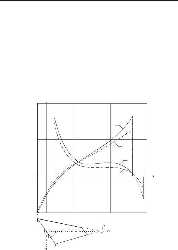
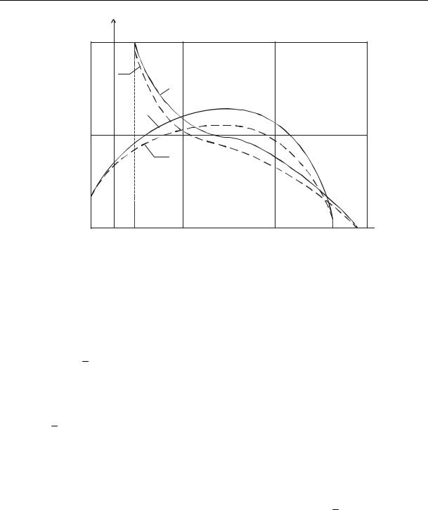
Some results of the numerical calculations for the model of the skew conic structure with a varying thickness with a rectangular contour of the transverse section are presented graphically. Fig. 2, 3 shows the character of the distribution of normal stresses z f (z) along the ribs of the upper panel ( y d1 / 2 ) under the impact of a rolling moment Mz = 392 N m at the end section (Fig. 2) and the bending force Qy = 588 N (Fig. 3).

Fig. 2. Distribution of normal stresses under the impact of a rolling moment

76

Fig. 3. Distribution of normal stresses under the impact of the bending force

constant thickness, the continuous ones are for a structure with a linear law of changes in the thickness at h h1 / h2 4 / 3. The graphs suggest that during rolling there is an edge effect both in the plane of the rigid embedding due to a restraint in warping of the contour and the end section due to the conic shape and changes in the thickness. As a relative thickness h h1 / h2 changes, the effect along the ends increases. Obviously, Fig. 3 needs no explanation. As for the effect of warping caused by bending on the stress-strain, as the numerical calculations suggest, it is actually insignificant and can be neglected in actual designing practice. Therefore the graphic dependencies are not presented.

In the limited transition to a structure with a constant thickness, i.e. at h 1, the results of numerical calculations are consistent with those presented in [7] and qualitatitvely agree with the experimental data for a similar structure presented in [1].

3. Solution with the use of the Wentzel-Kramers-Brillouin asymptotic method. Let us go back to the solution of the homogeneous differential equation (12) describing warping caused by rolling. This solution is written using the hypergeometric functions that are endless rows that do not agree much.

77

Russian Journal of Building Construction and Architecture

Let us now use the Wentzel-Kramers-Brillouin method according to which the solution of the equation (12) will be

where r 1. Making the coefficients for the identical degrees in (16) zero, we get an endless system of recurrent equations:

Intengrating the first equation of the system (17), we get the expression for the function of changeability:

(19) Then the second equation of the system (17) considering the solution (19) is significantly more simple:

78

ISSN 2542-0526

(21) Inserting (19) and (21) into (14), we get a general solution of the homogeneous equation (12):

U70 k /2 (C4 C5 ), (22)

where C4 ,C5 are integration constants determined using the boundary conditions of the task. Then using the variational method of the Lagrange constants we get a general integral of a homogeneous hypergeometric equation (12):

where H ( ) is a function of excitation that is the right part of the equation (11). The obtained solution (23) is much more simple than the above solution using hypergeometric functions and is more convenient to use on PC.

To conclude, let us note that the results of the calculation of the skew structure loaded with a concentrated moment Mz in the section z l1 obtained using the solution of the hypergeometric equation and the Wentzel-Kramers-Brillouin method are almost identical. The graphs are as presented in Fig. 2, 3.The latter suggests that the solution using the Wentzel-Kramers- Brillouin method is viable for practical calculations of weakly conic skew systems.

Conclusions. The paper presents the differences between the stress-strain of thin-walled spatial systems with a constant and varying thickness and this should be a consideration in the calculation of actual construction elements of bridge structures.

For the accepted and grounded assumptions the solution of the resolving system of regular differential equations was obtained not only numerically but also analytically using a tool of special functions and the Wentzel-Kramers-Brillouin method. This allows a qualitative analysis of the obtained solutions.

During rolling of the above thin-walled structure there is the edge effect both in the plane of a rigid embedding due to a restraint in warping of the contour and at the end section due to the conic shape and changes in the thickness. Considering warping of the transverse contour caused by bending does not have a significant effect on the stress-strain and can thus be neglected in actual designing practices.

References

1. Argiris Dzh. Sovremennye dostizheniya v metodakh rascheta konstruktsii s primeneniem matrits [Recent advances in methods of analysis of structures using matrix]. Moscow, Stroiizdat Publ., 1968. 240 p.

79

Russian Journal of Building Construction and Architecture

2.Beitmen G., Erdeii A. Vysshie transtsendentnye funktsii. Gipergeometricheskaya funktsiya. Funktsiya Lezhandra [Supreme transcendental functions. Hypergeometric function. The Function Of The Legendre]. Moscow, Nauka Publ., 1965. 294 p.

3.Galimov K. Z., Paimushin V. N. Teoriya obolochek slozhnoi geometrii [The theory of shells of complicated geometry]. Kazan, KGU Publ., 1985. 164 p.

4.Godunov S. K. O chislennom reshenii kraevykh zadach dlya sistem lineinykh obyknovennykh differentsial'nykh uravnenii [On numerical solution of boundary value problems for systems of linear ordinary differential equations]. Uspekhi matematicheskikh nauk, 1961, vol. XVI, iss. 3 (99), pp. 171—174.

5.Kamke E. Spravochnik po obyknovennym differentsial'nym uravneniyam [Handbook of ordinary differential equations]. Moscow, Nauka Publ., 1976. 703 p.

6.Kozlov V. A. Napryazhenno-deformirovannoe sostoyanie mnogosvyaznykh prizmaticheskikh konstruktsii, zakreplennykh po skoshennomu secheniyu [Stress-strain state of a multiply connected prismatic structures, mounted on a beveled cross section]. Nauchnyi vestnik Voronezhskogo GASU. Stroitel'stvo i arkhitektura, 2015, no. 4 (40), pp. 11—17.

7.Obraztsov I. F., Onanov G. G. Stroitel'naya mekhanika skoshennykh tonkostennykh system [Construction mechanics of beveled thin-walled systems]. Moscow, Mashinostroenie Publ., 1973. 660 p.

8. Kozlov V. A. Free vibrations of console restrained and prismatic thin-slab structures. Scientific Herald of the Voronezh State University of Architecture and Civil Engineering. Construction and Architecture, 2014, no. 3 (23), pp. 7—19.

9.Kozlov V. A. The Deflected Mode of Multi Coherent Prismatic Constructive Elements of Bridge Constructions. Scientific Herald of the Voronezh State University of Architecture and Civil Engineering, 2016, no. 3 (31), pp. 41—50.

10.Liu L., Liu G. R., Tan V. B. C. Element free method for static and free vibration analysis of spatial thin shell structures. Computer Methods in Applied Mechanics and Engineering, 2002, vol. 191, iss. 51—52, pp. 5923— 5942.

11.Piovan M. T., Cortinez V. H. Mechanics of thin-walled curved beams made of composite materials, allowing for shear deformability. Thin-Walled Structures, 2007, vol. 45, iss. 9, pp. 759—789.

12.Wang, Y., Liu Z., Wu H., Yan L. Spatial finite element analysis for dynamic response of curved thin-walled box girder bridges. Mathematical Problems in Engineering, 2016, vol. 2016. Available at: http://downloads.hindawi.com/journals/mpe/2016/8460130.pdf.

13.Seredin P. V., Glotov A. V., Domashevskaya E. P., Arsentyev I. N., Vinokurov D. A., Tarasov I. S. Raman investigation of low temperature AlGaAs/GaAs(1 0 0) heterostructures. Physica B: Condensed Matter, vol. 405, iss. 12, 15 June 2010, pp. 2694––2696. doi: 10.1016/j.physb.2010.03.049.

80