

Маслов ИНТРОДУЦТИОН ТО ПХЫСИЦС ОФ СЕЦОНД-ОРДЕР МАГНЕТИЦ 2015
.pdfWe have three solutions: ∆ = 0 and ∆ = ±
 2ab (TC −T ). Let us check the minimum condition, i.e., the positivity of second derivative
|
|
|
|
∂2 F (∆,T ) |
= 2a(T −T |
)+12b∆2 |
. |
|
(19.5) |
|||||
|
|
|
|
|
|
|
||||||||
|
|
|
|
∂∆2 |
|
|
C |
|
|
|
|
|
||
А. |
∆ = 0 |
|
∂2 F (∆,T ) |
= 2a(T −T |
)= |
> 0 at T |
>TC ; |
So, |
∆ = 0 is |
|||||
|
|
|
|
< 0 at T |
<T . |
|||||||||
∂∆2 |
||||||||||||||
|
|
|
|
C |
|
|
|
|
||||||
|
|
|
|
|
|
|
|
|
|
C |
|
|
||
the solution at |
T >TC (minimum), and it is not the solution at T <TC |
|||||||||
(maximum). |
|
|
|
|
|
|
∂2 F (∆,T ) |
|
|
|
B. ∆ = ± |
|
a |
(T |
−T ) |
= 4a(T −T )> 0 |
at T <T . So, |
||||
2b |
∂∆2 |
|||||||||
|
|
C |
|
|
C |
C |
||||
∆ ≠ 0 is the solution at T <TC (minimum). As this takes place, both ∆ > 0 and ∆ < 0 are the solutions, i.e., the ground state of the system at
T <TC is doubly degenerated. Therefore |
|
|||||||
|
( |
T |
) |
|
|
|
C |
|
∆ |
|
|
= |
0 at T >T ; |
(19.6) |
|||
∆ |
(T )− |
|
|
at T <TC , T →TC−. |
||||
T −TC |
||||||||
|
|
|
|
|
|
|
|
|
Finally, for all second-order phase transitions the temperature dependence ∆(T ) at T →TC has the same form, but ∆ has its own different physical meaning for each type of second-order phase transition.
20. Heat capacity of the Ising ferromagnet in the mean-field approximation
By definition |
|
|
dE (T ) |
|
|
|
|
|
||
|
C (T )= |
. |
|
|
|
(20.1) |
||||
|
|
|
|
|
||||||
At H = 0 |
|
|
dT |
|
|
|
|
|||
|
|
|
1 |
|
|
|
|
|
|
|
ˆ |
|
(T )− |
∑ |
/ |
Jij |
|
≈ |
|||
E (T )= H |
= E0 |
|
|
σiz σjz |
||||||
T |
|
|
|
2 i, j |
|
|
|
(20.2) |
||
≈ E0 (T )− x2 2(T )kBθN.
51

Therefore
C (T )= |
∂E |
0 (T ) |
− |
1 |
kBθN |
∂(x2 (T )) |
= C0 |
(T )+CS (T ), |
(20.3) |
|
∂T |
2 |
∂T |
||||||||
|
|
|
|
|
|
|||||
where C0 (T ) is the contribution to heat capacity which is not associated with magnetic ordering, and CS (T ) is the spin (magnetic) component. At T > θ the order parameter is x = 0 , therefore CS (T )= 0 C (T )= C0 (T ). At T < θ (T → θ− ) the order parameter is
|
|
|
|
|
|
|
|
|
|
|
|
|
|
|
|
|
|
|
x |
|
= 3 |
θ−T |
, thus x |
2 |
|
T |
. In this case |
|
|
||||||
|
|
|
|
||||||||||||||
|
|
θ |
|
= 3 1− |
|
|
|
|
|||||||||
|
|
|
|
|
|
|
|
θ |
|
|
|
|
|
|
|
||
|
|
|
|
|
|
CS |
(T )= − |
1 |
|
|
− |
3 |
|
3 |
kB N. |
(20.4) |
|
|
|
|
|
|
|
2 |
kBθN |
θ |
= |
2 |
|||||||
|
|
|
|
|
|
|
|
|
|
|
|
|
|
|
|||
Abrupt jump of heat capacity at T =θ |
is concerned with the appearance |
||||||||||||||||
new degrees of freedom in the system. So, at T > θ we have |
µˆ iz = 0 |
||||||||||||||||
i , and at T < θ we have  µˆ iz
µˆ iz  ≠ 0 i : the nonzero mean magnetic moments of all atoms are appeared. Every degree of freedom has, asso-
ciated with it, on an average, energy of |
|
1 kBT . At T →0 (T θ) the |
|||||||||||||||||||||||
|
|
|
|
|
|
|
|
|
|
|
|
2 |
|
|
|
|
|
|
|
|
|
|
|
|
|
|
|
|
=1− 2e−2 |
θ |
|
≈1− 4e−2 |
θ |
|
|
|
|
|
|
||||||||||||
order parameter is |
x |
T |
, thus x2 |
T |
. In this case |
||||||||||||||||||||
|
k |
|
θN |
|
−2 |
θ |
|
|
|
|
1 |
θ2 |
−2 |
θ |
|||||||||||
|
|
|
|
|
|
|
|
||||||||||||||||||
CS (T )= − |
|
B |
|
|
−4e |
|
|
T (−2θ) |
|
− |
|
|
|
|
= 4kB N |
|
|
e |
|
T . (20.5) |
|||||
|
|
|
|
T |
2 |
|
T |
2 |
|
||||||||||||||||
|
|
2 |
|
|
|
|
|
|
|
|
|
|
|
|
|
|
|
|
|
||||||
Therefore CS (T ) exponentially tends to zero at T →0 . |
|
|
|
|
|
|
|||||||||||||||||||
Generally speaking, |
C0 (T )≠ 0 |
|
thus |
total |
heat |
|
capacity |
||||||||||||||||||
C (T )= C0 (T )+CS (T ) |
takes the form as it is shown on Fig. 20.1, i.e. at |
||||||||||||||||||||||||
T = θ the abrupt jump takes place ∆C = |
3 k |
B |
N. |
|
|
|
|
|
|
||||||||||||||||
|
|
|
|
|
|
|
|
|
|
|
2 |
|
|
|
|
|
|
|
|
|
|
|
|
||
52

Fig. 20.1. Temperature dependence of ferromagnet heat capacity in the mean-field approximation
Note that for the heat capacity the mean-field approximation gives qualitatively wrong result. As we can see, mean-field approximation predicts the abrupt jump for heat capacity, but in fact it has divergence
C (T )− T −θ−α (see Fig. 20.2).
Fig. 20.2. Realistic temperature dependence of ferromagnet heat capacity
Such characteristic feature of the Ising ferromagnet heat capacity is called lambda point.
53

21. Magnetic susceptibility of the Ising ferromagnet in the mean-field approximation
Recall |
the definition of the differential magnetic |
susceptibility |
||
χ = (∂M ∂H )H →0 . In |
paramagnetic |
state (T > θ) the |
magnetization |
|
M = 0 at |
H = 0 and |
M ≠ 0 only at |
H ≠ 0 . In this case “conventional” |
|
magnetic susceptibility χ = M H coincides with the differential one.
Earlier we showed that at |
T θ magnetic susceptibility could be de- |
||||
scribed as χ = |
NµB2 |
1 |
|
(Curie-Weiss law). Let us find the expression |
|
V |
|
T −θ |
|
||
for χ(T ) in all temperature range 0 <T < +∞. What should we do? We must obtain the M (H ) dependence and differentiate it with respect to
H . We know that M = NVµB x (see Eq. (12.6)), thus we should find the dependence x(H ). It can be found from the Curie-Weiss equation with
regard to magnetic field |
|
x = tanh |
h + xθ |
. Since in this equation we |
|||||||||||||||||||||||||||||
|
|
T |
|
|
|
||||||||||||||||||||||||||||
|
|
|
|
|
|
|
|
|
|
|
|
|
|
|
|
|
|
|
|
|
|
|
|
|
|
|
|
|
|
|
|
||
have h rather than H , let us make the following conversion |
|
||||||||||||||||||||||||||||||||
|
|
|
|
|
|
|
|
|
|
|
|
|
∂M |
|
|
|
Nµ2 |
∂x |
|
|
|
|
|
|
|
|
|||||||
|
|
|
|
|
|
χ = |
|
|
|
= |
|
|
|
B |
|
|
|
. |
|
|
|
|
|
(21.1) |
|||||||||
|
|
|
|
|
|
∂H |
|
|
V |
|
∂h |
|
|
|
|
|
|||||||||||||||||
|
|
|
|
|
|
|
|
|
|
|
|
|
|
|
|
|
|
|
h→0 |
|
|
|
|
|
|
||||||||
Considering that we do not know the dependence x(h) |
let us differenti- |
||||||||||||||||||||||||||||||||
ate the both sides of the Curie-Weiss equation |
|
|
|
|
|
|
|
||||||||||||||||||||||||||
∂x |
|
2 h + xθ |
|
|
|
|
1 |
|
|
θ ∂x |
|
|
1 |
− x2 |
|
θ |
(1− x |
2 |
) |
∂x |
|
||||||||||||
|
= 1− tanh |
|
|
|
|
|
|
|
|
|
+ |
|
|
|
|
|
|
= |
|
|
|
+ |
|
|
|
; |
|||||||
∂h |
T |
|
|
|
T ∂h |
|
T |
T |
|
∂h |
|||||||||||||||||||||||
|
|
|
|
|
T |
|
|
|
|
|
|
|
|
|
|
|
|||||||||||||||||
|
|
|
∂x |
1 |
− |
|
θ |
|
(1− x2 ) = 1− x2 |
; |
|
|
|
|
|
|
(21.2) |
||||||||||||||||
|
|
|
|
|
|
|
|
|
|
|
|
||||||||||||||||||||||
|
|
|
∂h |
|
|
T |
|
|
|
|
|
|
|
|
|
|
|
|
|
T |
|
|
|
|
|
|
|
|
|
||||
|
|
|
|
|
∂x |
|
= |
|
|
|
|
|
1 |
− x2 |
|
|
. |
|
|
|
|
|
|
|
|
|
|||||||
|
|
|
|
|
∂h |
|
|
|
|
|
|
( |
|
|
|
|
) |
|
|
|
|
|
|
|
|
|
|||||||
|
|
|
|
|
|
|
|
|
|
|
|
|
|
|
|
|
|
|
|
|
|
|
|
|
|
|
|
||||||
|
|
|
|
|
|
|
|
|
T −θ 1− x |
|
|
|
|
|
|
|
|
|
|
|
|
||||||||||||
|
|
|
|
|
|
|
|
|
|
|
|
|
|
|
|
|
|
|
|
|
2 |
|
|
|
|
|
|
|
|
|
|
|
|
54

Here we take into account that
∂tanh z |
= |
∂ sinh z |
= |
cosh2 z −sinh2 z |
=1− tanh |
2 |
z. |
|||||||
|
|
|
|
|
|
|
|
|
|
|
||||
∂z |
|
|
cosh |
2 |
z |
|
|
|
||||||
|
∂z cosh z |
|
|
|
|
|
|
|
|
|||||
Therefore the expression for χ(T ) takes the following form |
|
|
||||||||||||
|
|
|
χ = |
NµB2 |
|
1− x2 |
|
|
|
. |
|
|
(21.3) |
|
|
|
|
V |
|
|
T −θ 1− x2 |
) |
|
|
|||||
|
|
|
|
|
|
( |
|
|
|
|
|
|
||
Further we should tend the magnetic field to zero, i.e., take as order parameter the solution of the Curie-Weiss equation without H :
xθ |
. We already know this solution and in limiting cases at |
|||
x = tanh |
|
|
||
T |
||||
|
|
|
||
T →0 and at T < θ (T → θ− ). Let us analyze the Eq. (21.3).
A. At T > θ the order parameter is x = 0 χ = |
NµB2 |
1 |
. Thus we |
|
V |
|
T −θ |
||
obtain the Curie-Weiss law. Therefore the Curie-Weiss law is correct in all temperature range T > θ inclusive T = θ, i.e., the magnetic susceptibility is diverged at T → θ+ . So, the magnetization itself is finite, but its
rate of change becomes infinite at H → 0 and T →θ.
|
|
|
|
|
|
|
|
|
|
|
|
|
|
|
|
|
|
|
|
|
|
|
|
|
|
|
T |
||
B. At T → θ− |
the order parameter is |
|
|
x |
|
= 3 |
θ−T |
x |
2 |
|
− |
||||||||||||||||||
|
|
|
|
||||||||||||||||||||||||||
|
|
|
|
|
|
|
= 3 1 |
. |
|||||||||||||||||||||
In this case |
|
|
T |
|
|
|
|
|
|
|
|
|
|
|
|
|
|
|
θ |
|
|
|
|
|
|
|
|
θ |
|
|
|
|
|
|
|
|
|
|
|
|
|
|
|
|
|
|
|
|
|
|
|
|
|
|
|
|
|||
|
|
|
|
|
|
|
|
|
|
|
|
|
|
|
|
|
|
|
|
|
|
|
|
|
|
|
|
|
|
χ = |
NµB2 |
|
|
3 θ − 2 |
|
≈ |
NµB2 |
|
|
|
|
1 |
|
|
|
= |
NµB2 |
|
|
|
1 |
|
. |
|
|||||
V |
|
T |
|
T |
− 2 |
|
V T |
− |
3T |
+ θ |
V 2 |
( |
θ− |
T ) |
|
||||||||||||||
|
|
−θ 3 |
θ |
|
|
|
|
2 |
|
|
|
|
|
||||||||||||||||
|
|
|
|
|
|
|
|
|
|
|
|
|
|
|
|
|
|
|
|
|
|
|
|
|
|
|
|
|
|
So, at T → θ− |
|
magnetic susceptibility is also diverged, and the charac- |
|||||||||||||||||||||||||||
ter of divergence is the same that at T → θ+ . Let us unify our results at T → θ− and at T → θ+
χ(T )− |
1 |
|
|
at T → θ. |
(21.4) |
|
|
T −θ |
|
|
|||
|
|
|||||
|
|
|
|
|
|
|
55
C. At T →0 (T θ) the order parameter is
|
|
|
|
|
≈1− 2e−2 |
θ |
x2 ≈1− 4e−2 |
θ |
|
||||||||||||
|
|
|
x |
|
|
|
. |
|
|
||||||||||||
In this case |
|
|
T |
T |
|
||||||||||||||||
|
|
|
|
|
|
|
|
|
|
|
|
|
|
|
|
|
|
|
|
|
|
|
|
|
NµB2 |
|
4e−2 |
θ |
|
|
|
|
NµB2 4e−2 |
θ |
|
||||||||
χ = |
|
|
|
T |
|
|
|
≈ |
T |
. |
|||||||||||
|
|
|
|
|
|
|
|
|
|
|
|
|
|
T |
|||||||
|
|
|
|
V |
|
T −θ |
|
4e |
−2 |
θ |
|
V |
|||||||||
|
|
|
|
|
|
|
|
||||||||||||||
|
|
|
|
|
|
|
|
|
T |
|
|
|
|
|
|
||||||
|
|
|
|
|
|
|
|
|
|
|
|
|
|
|
|
|
|
|
|
||
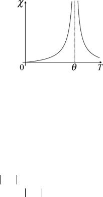
Thus the magnetic susceptibility exponentially tends to zero at T →0. The resulting temperature dependence of χ is shown on Fig. 21.1.
Fig. 21.1. Temperature dependence of ferromagnet magnetic susceptibility
Why is the magnetic susceptibility tend to zero at T →0 and at T →∞ ? The reason is that in both cases it is nothing to ordering: at T →0 all the magnetic moments are already ordered (even without a magnetic field), and at T →∞ atoms do not have the mean magnetic moments.
22. Critical exponents
We obtained that at T → θ the magnetic susceptibility diverged by the law χ(T )− T −θ−1 (see § 21), and order parameter has the squareroot singularity ∆(T )− T −θ1/2 at T → θ− (see § 19). As for heat ca-
56
pacity, in the mean-field approximation it has the abrupt |
jump (see |
||||||||
§ 20). Critical exponents α , β and γ are denoted as follows |
|
||||||||
C (T )− |
|
|
|
T −θ |
|
|
|
−α ; |
|
|
|
|
|
|
|||||
∆(T )−(T −θ)β ; |
(22.1) |
||||||||
χ(T )− |
|
T −θ |
|
−γ . |
|
||||
|
|
|
|||||||
In the case of ferromagnetic phase transition in the mean-field approximation we have α = 0 , β = 12 and γ =1. Let us compare these results
with the numerical calculations (3D Ising model) and experimental data (see Table 22.1).
Table 22.1
Critical exponents obtained using mean-field approximation and numerical calculations along with experimental data
Critical exponent |
Mean-field |
Numerical |
Experiment |
|
approximation |
calculations |
|||
|
|
|||
α |
0 |
0,12 |
≈ 0,1 |
|
|
|
|
|
|
β |
0,5 |
0,31 |
0,3 ÷0,4 |
|
|
|
|
|
|
γ |
1 |
1,25 |
1,2 ÷1,4 |
|
|
|
|
|
|
α + 2β + γ |
2 |
1,99 |
1,9 ÷2,3 |
|
|
|
|
|
Overall, there are about ten different critical exponents, but some of them depend on each other. It can be exactly shown that (see Table 22.1)
α + 2β+ γ = 2 . |
(22.2) |
In the mean-field approximation the expression mentioned above is also correct, but unfortunately each exponent separately is incorrect.
23. Exact solution of the Ising model in one dimension
Recall that the |
Curie temperature, by definition, is |
θ = ∑J (Rl )= zJ, where |
z is the number of nearest neighbors of each |
Rl ≠0 |
|
57
atom. In the formula for θ we denote the J (Rl )= J > 0 for the nearest
neighbors and consider the J (Rl )= 0 for other atoms. Therefore, for
the one-dimensional chain of magnetic moments the mean-field approximation predicts the ferromagnetic phase transition at θ = 2J (if the interactions between only nearest neighbors are taken into account). Let us solve the problem for one-dimensional chain of magnetic moments with interactions only between the nearest neighbors exactly. The Hamiltonian in the Ising model is
|
|
|
|
= − |
1 |
∑ |
/ |
|
|
|
(23.1) |
|
|
|
H |
|
|
Jij σiz σjz |
− h∑σiz , |
||||
|
|
|
|
|
2 i, j |
|
|
|
i |
|
|
|
|
|
|
|
|
|
|
|
|
|
|
µiz |
, |
h = µB H , and |
|
σiz |
= ±1 are the eigenvalues of opera- |
||||||
where σiz = |
µB |
|
|||||||||
|
|
|
|
|
|
|
|
|
|
|
|
tors σiz . Note again that the interaction occurs only between the nearest neighbors, so, Jij = J > 0 if i and j are the numbers of the nearest mag-
netic moments and Jij = 0 otherwise. Let us numerate all the magnetic
moments in the system from “1” to “N”. Therefore the Hamiltonian takes the form
|
|
|
|
|
|
|
|
(23.2) |
H |
= −J σ1z σ2z − J σ2z σ3z −... − J σN −1,z σNz − h(σ1z +... + σNz ). |
|||||||
Since |
N 1 the boundary conditions are not essential. Let us make |
|||||||
them periodical, i.e., “close the chain into the ring”. In other words, we add into the Hamiltonian between the 1-st and N-th magnetic moments
the following term |
−J |
|
|
|
|
|||
σNz σ1z . Next, let us calculate the partition func- |
||||||||
|
ˆ |
|
|
|
|
En |
|
|
|
−H |
|
∑ |
|
− |
|
||
|
|
= |
e T |
|
, where n are the numbers of the Hamiltoni- |
|||
tion Q =Tr e |
T |
|
|
|||||
|
|
|
n |
|
|
|
|
|
an eigenstates and En are the corresponding energies. If we know the partition function, we can calculate the free energy F = −T lnQ , and finally – the order parameter x.
58

|
Every state “n” is defined by the set of N numbers σiz |
|
|
each is equal |
||||||||||||||||||||||||||||
+1 or –1, and ∑ is the sum over all number sets {σiz } |
|
|
|
|||||||||||||||||||||||||||||
|
|
n |
|
|
|
|
|
|
|
|
|
|
|
|
|
|
|
|
|
|
|
|
|
|
|
|
|
|
|
|
|
|
|
|
|
|
|
|
|
|
|
|
|
|
|
|
|
|
|
|
ˆ |
|
|
|
|
|
|
|
|
|
|
|
|
|
|
|
|
|
|
|
|
|
|
|
|
|
|
|
|
|
|
|
|
H |
|
|
|
|
|
|
|
|
|
|
|
|
|
|
|
|
|
|
|
|
|
Q = ∑ |
{σiz } |
|
e− T |
|
|
{σiz } . |
|
|
|
|
(23.3) |
||||||||||||||
|
|
|
|
|
|
|
|
|
|
|
|
|
||||||||||||||||||||
|
|
|
|
|
|
|
|
|
|
{σiz } |
|
|
|
|
|
|
|
|
|
|
|
|
|
|
|
|
|
|
|
|
|
i =1,..., N , |
The Hamiltonian |
|
|
is |
|
the function |
|
of |
|
operators |
, |
||||||||||||||||||||||
|
|
|
|
|
σiz |
|||||||||||||||||||||||||||
ˆ |
|
|
|
). Since |
|
|
{σiz } |
|
|
= σkz |
|
{σiz } |
k , then |
|||||||||||||||||||
|
|
|
|
|||||||||||||||||||||||||||||
H |
= H (σ1z ,σ2z ,...,σNz |
σkz |
|
|
|
|||||||||||||||||||||||||||
|
|
|
ˆ |
|
{σiz } |
= H (σ1z ,σ2z ,...,σNz ){σiz } . |
|
|
|
|||||||||||||||||||||||
|
|
|
|
|
|
|
||||||||||||||||||||||||||
|
|
H |
|
|
|
|
||||||||||||||||||||||||||
Therefore |
|
|
|
|
|
|
|
|
|
|
|
|
|
|
|
|
|
|
|
|
|
Nz ) |
|
|
|
|
|
|
|
|
||
|
|
|
|
|
ˆ |
|
|
|
|
|
|
H |
σ |
,σ |
2 z |
,...,σ |
|
|
|
|
|
|
|
|
||||||||
|
|
|
|
|
H |
|
|
|
|
|
|
|
( 1z |
|
|
|
|
|
|
|
|
|
|
|
|
|||||||
|
|
|
e− T |
|
{σiz } = e− |
|
|
|
|
|
|
|
|
|
|
|
|
{σiz } . |
|
|
|
|
||||||||||
|
|
|
|
|
|
|
|
|
T |
|
|
|
|
|
|
|
|
|
|
|||||||||||||
Considering these expressions, for the partition function we obtain |
||||||||||||||||||||||||||||||||
|
|
Q = ∑ |
{σiz } |
|
e− |
H (σ1z ,...,σNz ) |
|
{σiz } |
= ∑e− |
H (σ1z ,...,σNz ) |
= |
|||||||||||||||||||||
|
|
|
T |
|
|
|
|
T |
|
|
||||||||||||||||||||||
|
|
{σiz } |
|
|
|
|
|
|
|
|
|
|
|
|
|
|
|
|
|
|
|
|
{σiz } |
|
|
|
|
(23.4) |
||||
|
|
|
|
|
|
|
|
|
|
|
|
|
|
|
|
|
|
|
|
|
|
|
|
|
|
|||||||
|
|
|
|
|
|
|
|
|
|
|
|
|
|
|
|
|
|
|
|
|
H (σ1z ,...,σNz ) |
|
|
|
|
|||||||
|
|
|
|
|
= ∑ ∑ |
... ∑ e |
− |
, |
|
|
|
|
||||||||||||||||||||
|
|
|
|
|
|
|
T |
|
|
|
|
|
|
|
||||||||||||||||||
|
|
|
|
|
|
|
|
|
|
|
|
|
|
|
|
|||||||||||||||||
|
|
|
|
|
|
|
|
|
|
|
|
|
|
|
|
|
|
|
|
|
|
|
|
|
|
|
|
|
|
|
||
σ1z =±1 σ2 z =±1 σNz =±1
where
H (σ1z ,...,σNz )= −Jσ1z σ2z − Jσ2z σ3z −... − JσN −1,z σNz − JσNz σ1z − −hσ1z − hσ2z −... − hσNz .
So,
|
|
|
|
J |
|
|
|
|
J |
|
|
|
J |
|
|||
Q = ∑ |
... ∑ exp |
|
|
σ1zσ2z |
+ |
|
σ2zσ3z +... + |
|
|
σN −1,zσNz + |
|||||||
|
|
T |
T |
||||||||||||||
σ1z =±1 σNz =±1 |
T |
|
|
|
|
|
|
|
|
||||||||
|
|
J |
|
|
|
|
h |
|
|
h |
σ2z +... + |
h |
|
|
|
||
|
+ |
|
σNzσ1z + |
|
|
σ1z + |
|
|
|
σNz |
= |
||||||
|
T |
T |
|
T |
T |
||||||||||||
|
|
|
|
|
|
|
|
|
|
|
|
||||||
59
|
|
|
|
J |
|
|
|
|
|
|
|
|
|
|
|
h |
|
|
|
|
|
|
|
|
|
|
|
|
|
|
|
|
|
J |
|
|
|
|
||
= ∑ ... ∑ exp |
|
σ1z σ2z |
+ |
|
|
|
|
(σ1z + σ2z )+ |
|
σ2z σ3z |
+ |
|||||||||||||||||||||||||||||
|
2T |
|
|
T |
||||||||||||||||||||||||||||||||||||
σ1z =±1 σNz =±1 |
T |
|
|
|
|
|
|
|
|
|
|
|
|
|
|
|
|
|
|
|
|
|
|
|
|
|
|
|
|
|
|
|
|
|||||||
+ |
h |
(σ2z |
+ σ3z )+... + |
|
|
J |
|
σN −1,z σNz + |
|
|
|
|
||||||||||||||||||||||||||||
2T |
|
|
|
|
|
|
|
|
|
|||||||||||||||||||||||||||||||
|
|
|
|
|
|
|
|
|
|
|
|
|
|
|
|
|
|
|
|
|
T |
|
|
|
|
|
|
|
|
|
|
|
|
|||||||
+ |
h |
(σN −1,z + σNz )+ |
|
J |
|
σNz σ1z + |
|
h |
(σNz + σ1z ) . |
|
||||||||||||||||||||||||||||||
|
|
T |
|
|
2T |
|
||||||||||||||||||||||||||||||||||
|
2T |
|
|
|
|
|
|
|
|
|
|
|
|
|
|
|
|
|
|
|
|
|
|
|
|
|
|
|
|
|
|
|
||||||||
Denote the 2 ×2 matrix A |
|
|
|
|
|
|
|
|
|
|
|
|
|
|
|
|
|
|
|
|
|
|
|
|
|
|
|
|
|
|
|
|
|
|
|
|||||
|
|
|
|
|
A = |
|
|
A |
|
|
|
|
|
|
A |
|
|
|
|
|
|
|
|
|
|
|
|
|
|
(23.5) |
||||||||||
|
|
|
|
|
|
|
1,1 |
|
|
|
|
|
1,−1 |
, |
|
|
|
|
|
|
|
|||||||||||||||||||
|
|
|
|
|
|
|
|
A |
|
|
|
|
|
A |
|
|
|
|
|
|
|
|
|
|
|
|
|
|
|
|
|
|||||||||
|
|
|
|
|
|
|
|
|
−1,1 |
|
|
|
−1,−1 |
|
|
|
|
|
|
|
|
|||||||||||||||||||
where the matrix elements are |
Aσ |
,σ |
|
= exp |
J |
|
σ1z σ2z + |
|
h |
(σ1z + σ2z ) . |
||||||||||||||||||||||||||||||
2 z |
|
|
|
|
||||||||||||||||||||||||||||||||||||
|
|
|
|
|
|
|
|
|
|
1z |
|
|
|
|
|
|
|
|
|
|
|
|
|
|
|
|
|
|
|
|
|
|
|
2T |
|
|||||
Thus the matrix takes the following form |
|
|
|
|
|
|
|
T |
|
|
|
|
|
|
||||||||||||||||||||||||||
|
|
|
|
|
|
|
|
|
|
|
|
|
|
|
|
|
|
|||||||||||||||||||||||
|
|
|
|
|
|
|
|
|
|
J |
+ |
h |
|
|
|
|
|
− |
J |
|
|
|
|
|
|
|
|
|
|
|
||||||||||
|
|
|
|
|
|
|
eT |
|
|
T |
|
|
e |
|
T |
|
|
|
|
|
|
|
|
(23.6) |
||||||||||||||||
|
|
|
|
|
A = |
|
|
|
|
J |
|
|
|
|
|
J |
|
|
h |
. |
|
|
|
|
|
|
|
|||||||||||||
|
|
|
|
|
|
|
|
|
e− |
|
|
|
|
e |
|
− |
|
|
|
|
|
|
|
|
|
|
||||||||||||||
|
|
|
|
|
|
|
|
T |
|
|
|
T |
T |
|
|
|
|
|
|
|
|
|||||||||||||||||||
Denote the other matrix elements Aσ |
2 z |
,σ |
|
|
|
|
,..., Aσ |
Nz |
,σ |
in the same way. |
||||||||||||||||||||||||||||||
For Q we obtain |
|
|
|
|
|
|
|
|
|
|
|
|
|
|
|
|
|
|
3 z |
|
|
|
|
|
1z |
|
|
|
|
|
||||||||||
|
|
|
|
|
|
|
|
|
|
|
|
|
|
|
|
|
|
|
|
|
|
|
|
|
|
|
|
|
|
|
|
|
|
|
|
|
||||
Q = ∑ ... ∑ Aσ1z ,σ2 z |
|
Aσ2 z ,σ3 z ,..., AσN −1,z ,σNz |
AσNz ,σ1z . |
(23.7) |
||||||||||||||||||||||||||||||||||||
|
σ1z =±1 σNz =±1 |
|
|
|
|
|
|
|
|
|
|
|
|
|
|
|
|
|
|
|
|
|
|
|
|
|
|
|
|
|
|
|
|
|
|
|
||||
Recall the rule of matrix multiplication (A2 )kn = ∑Akm Amn . Therefore |
|||||||||||||
∑ Aσ1z ,σ2 z |
|
|
= (A2 )σ |
|
m |
|
|||||||
Aσ2 z ,σ3 z |
|
,σ |
3 z |
, |
|||||||||
σ2 z =±1 |
|
|
|
|
|
|
|
1z |
|
|
|
||
∑ (A2 )σ |
,σ |
3 z |
Aσ3 z ,σ4 z |
= (A3 )σ |
,σ |
|
, …, |
||||||
σ3 z =±1 |
1z |
|
|
|
|
|
1z |
|
|
4 z |
|
||
∑ (AN −1 )σ |
,σ |
AσNz ,σ1z = (AN )σ |
,σ . |
||||||||||
σN ,z =±1 |
|
|
1z |
|
Nz |
|
|
|
|
|
|
1z |
1z |
|
|
|
|
|
|
|
|
|
|
|
|
|
|
Finally, for the partition function we obtain |
|
|
|
|
|
|
|||||||
|
Q = ∑ (AN )σ |
, |
σ . |
|
|
|
|
(23.8) |
|||||
|
|
|
σ1z =±1 |
1z |
|
1z |
|
|
|
|
|
||
|
|
|
|
|
|
|
|
|
|
|
|||
60