- •1. Electrostatic field. Coulomb’s law. Gauss law (Электростатическое поле. Закон Кулона. Закон Гаусса)
- •Variables and units
- •Coulomb’s Law. (ЗаконКулона)
- •Electric Field Strength e and Displacement Field d. (Напряжённостьисмещениеэлектрическогополя)
- •Gauss’ Law. (ЗаконГаусса)
- •2. Poisson’s and Laplace’s equations for the potential of electric field (Уравнения Пуассона и Лапласа для потенциала электрического поля) Electric Potential. (Электрический потенциал)
- •Poisson’s and Laplace’ s equations. (Уравнения Пуассона и Лапласа)
- •3. Electrostatic Energy (Электростатическая энергия) Electrostatic Energy (Электростатическаяэнергия)
- •Virtual experiment. (Эксперимент по нахождению энергии системы)
- •Consequences (Следствия)
- •4. Power and Joule’s Law (Энергия и закон Джоуля-Ленца)
- •5. Continuity Equation (Уравнения непрерывности) ContinuityEquation (Уравнение непрерывности)
- •Image method for the flat boundary between magnetic media (Метод изображений для плоской границы между магнитными носителями)
- •8. Static magnetic field. Biot–Savart’s Law. Ampere’s Law (Статическое магнитное поле. Закон Био–Савара. Закон Ампера)
- •Variables and units (Переменные и единицы измерения)
- •Main Relations (Основные соотношения)
- •Magnetic flux density (Индукция магнитного поля)
- •Biot-Savart’s law (Закон Био-Савара)
- •Ampere’s law (Закон полного тока)
- •The cut in the space (Разрез в пространстве)
- •Laplace equation for the scalar magnetic potential (Уравнение Лапласа для скалярного магнитного потенциала)
- •10. Vector magnetic potential. Inductance (Векторный магнитный потенциал. Индуктивность)
- •Vector magnetic potential (Векторный магнитный потенциал)
- •Magnetic flux (Магнитный поток)
- •Differential equation for the vector magnetic potential (Дифференциальное уравнение для векторного магнитного потенциала)
- •Gauging of the vector magnetic potential (Калибровка векторного магнитного потенциала)
- •Integral presentation of the vector magnetic potential (Интегральное представление векторного потенциала)
- •Inductance (Индуктивность)
- •Mutual inductance (Взаимная индуктивность)
- •Inductance of thin contours (Индуктивность тонких контуров)
- •12. Internal inductance of a thin conductor (Внутренняя индуктивность тонкого проводника) Flux linkage of a thin current layer (Потокосцепление тонкого слоя с током)
- •Internal inductance of a thin conductor (Внутренняя индуктивность тонкого проводника)
- •13. Inductance of a two wire transmission line (Индуктивность двухпроводной линии).
- •14. Variable separation method in a cylindrical coordinate system (Метод разделения переменных в цилиндрической системе координат). Application of Laplace’s equation (Применение уравнения Лапласа).
- •Angular function (Угловая функция)
- •Radial function (Радиальная функция)
- •General solution of the Laplace’s equation in a cylindrical coordinate system (Общее решение уравнения Лапласа в цилиндрической системе координат)
- •15. The Faraday’s law (Закон электромагнитной индукции).
- •Lenz’s Law (правило Ленца)
- •Induction by a temporal change of b (Индукция за счёт временного изменения b)
- •16. Induction through the motion of a conductor (Индукция за счет движения проводника).
- •17. Induction by simultaneous temporal change of b and motion of the conductor (Индукция одновременным изменением b во времени и движением проводника).
- •18. Unipolar generator (Униполярный генератор).
- •19. Hering’s paradox (Парадокс Геринга)
- •20. Diffusion of magnetic fields into conductors (Распространение электромагнитного поля в проводнике)
- •21. Periodic electromagnetic fields in conductors. (Периодическое электромагнитное поле в проводниках)
- •Penetration of the electromagnetic field into a conductor. (Проникновение электромагнитного поля в проводник)
- •The skin effect. (Скин-эффект)
- •22. Poynting theorem. (Теорема Пойнтинга) Electromagnetic Field Energy. (Энергия электромагнитного поля)
- •The rate of decrease of the electromagnetic field energy in a closed volume. (Скорость уменьшения энергии электромагнитного поля в замкнутом объёме)
- •Transmission of energy in a dc line (Передача энергии в линиях постоянного тока)
- •The field picture near the wires with current (Картина поля вблизи провода с током)
- •25. Energy flows in static electric and magnetic fields (Поток энергии в статических электрических и магнитных полях).
- •26. The reduced magnetic potential (Редуцированный магнитный потенциал). Reduced scalar magnetic potential (Редуцированный скалярный магнитный потенциал)
- •Combination of scalar magnetic potential and reduced magnetic potential (Комбинация скалярного магнитного потенциала и редуцированного магнитного потенциала)
- •27. Classification of numerical methods of the electromagnetic field modeling (Классификация численных методов моделирования электромагнитного поля).
- •Classification of the problems (Классификация проблем)
- •Classification of the methods (Классификация методов)
- •28. Method of moments
- •Discretization of the problem domain (Дискретизация проблемной области)
- •29. Basic principles of the finite element method.
- •30. Finite functions (Ограниченная функция – отлична от нуля только в пределах треугольника)
- •Simplex coordinates
- •Approximation of functions inside triangles (Аппроксимация функций внутри треугольника)
- •Approximation of the equation (Аппроксимация уравнения)
- •31. Weighted residual method (метод взвешенных невязок)
- •32. Weak formulation of the electromagnetic field modeling problem
- •33. Boundary conditions in electric and magnetic fields
- •1) First type boundary conditions
- •34. Main equations of electromagnetic field in integral form.
- •35. Main equations of electromagnetic field in differential form.
- •36. Electric field of a point charge (Электрическое поле точечного заряда)
- •37. Electric field of a uniformly charged sphere (Электрическое поле равномерно заряженной сферы)
- •38. Flat capacitor. Field. Surface charge. Capacity. (Плоский конденсатор. Поле. Поверхностный заряд. Вместимость.)
- •39.2 Inductance of a cylindrical coil with the rectangular cross section(Индуктивность цилиндрической катушки прямоугольного сечения).
- •4 0.1 Electric field induced by charged line placed above conducting surface (Электрическое поле, создаваемое заряженной линией, помещенной над проводящей поверхностью).
- •4 0.2. Magnetic field induced by the line with a current placed above a ferromagnetic surface with infinitely high magnetic permeability
32. Weak formulation of the electromagnetic field modeling problem
Let’s remember what it is, an integration-by-part. The initial equation is:
Inside the Galerkin method we decide that this integral is equal to zero:
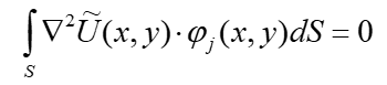
At the same time the approximation of the potential is the first function:
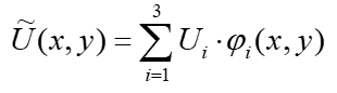
So, the coefficient Ui is constant, so it can be moved outside the integral, also a sign of sum can be moved outside the integral. So we get next equation:
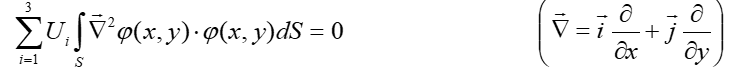
Now it is the second order derivative, that is Laplacian, which is applied to the finite function of the first order. Until now, in any case this integral will give us zero, because this is the first order polynomial.
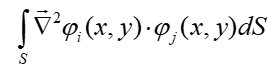
Let’s look to the possible transformations. Let’s consider separately this integral:
For this purpose we shall use a relation from vector algebra:
Now let’s assume and . So:
So, we can express:
These functions are under the integral now let’s apply integral operator to this expression. What shall we get?
Integrating the last relation over the problem domain:
We can use the Gauss theorem:
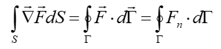
Instead of the first term in the right part we can use the integral over the boundaries (Г is an element of the surface). So, we can express the integral from the Laplacian of the finite function times finite function by these two expressions:
Г is the border of the problem domain, it is not the border of triangle. Our integrations may be considered as integration over the whole domain. So, this integral is equal to zero everywhere inside the problem domain. That’s why for a certain triangle we can say:
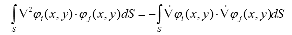
That is a very important transformation, now under the right integral we have two functions, which are not equal to zero, and this integral has the certain value. Of course, it is very unpleasant expression, expression under the left integral is equal to zero by default, so, it looks like this integral is equal to zero, on the other hand, we found out that it is not equal to zero at all. How to explain it? The explanation is very simple, really function φ so called finite function is not continuous, it jumps from a certain value to zero at the border element, and so it is not simple to understand what will give this jump, how to include it into relations. First of all, what is important the first impression - left integral is equal to zero, the second impression, probably it may differ from zero, but it's very difficult to define what is the value of this integral, if we shall take into account the jump of the function from certain value to zero. What does mean that jump? The derivative is equal to infinity, the second order derivative is certainly infinitely big, that’s why the integral even over very small area associated with the sides of triangle, with the edges of triangle, in principle not necessary will be equal to zero. So, this is general consideration, it’s very difficult to answer the question how to calculate this integral for us it’s very important. We have found an exact value of the left integral and now we can calculate it.
So, instead the initial integral, which include the second order derivative of the function we have now got a similar equation, but now under the integral we have a product of two gradients, two gradients are two constants inside a triangle.
Again, coefficients are the potentials, if we are talking about the certain triangle, instead of N we should write 3 nodes. Ui - this are the unknown potentials; from the beginning we do not know what the values of these potentials are. Integrals are very interesting, because we can calculate them before we shall start to solve the problem. Indeed, we know the finite function inside each triangle, this finite function does not depend on a final solution, it is property of the triangle. So, we can find a gradient of the finite function, we can find a product of 2 gradients and certainly we can integrate this product over the area. Finally, we have a system of equations of this form, where the coefficients are simply the integrals, which may be calculated independently on the soft problem, that is the problem only of the dimensions, positions of triangles:
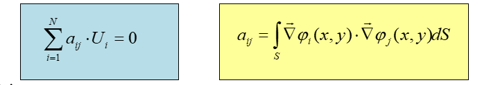
If we shall apply this idea not for one triangle but for many triangles inside certain mesh, then number of unknowns will be equal to the total number of the nodes inside this mesh. So, this is the main idea behind the finite element method, this is so-called weak formulation. Why is it called weak formulation? Coming back to the initial area,
If we shall try to exactly solve this equation applying the second order derivative, Laplacian operator to the approximate value of the potential, then it will be strong formulation, we are looking exactly for the function, which is used for the potential approximation. But after this integration-by-part we have used some additional mathematical properties of this transformation and now we are looking for solutions for the different equations, and that is called weak formulation of the Galerkin method, of the weighted residual method.
If the boundary potentials are known in advance, several equations in the system will have non-zero right hand sides.