27. Classification of numerical methods of the electromagnetic field modeling (Классификация численных методов моделирования электромагнитного поля).

There are two different items, that are used for this classification. First of them, evidently the use the method depends strongly on the problem, which it solves. That is why first classification is classification of the problems.

Classification of the problems (Классификация проблем)

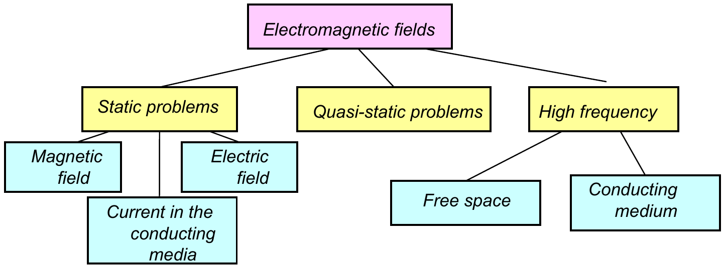
• Static problems – do not depend on time (DC current in the conducting media). This problem is differing from the electrostatics. We already define what is it electrostatics. First property of this field is absenting of the time dependent fields and there are no currents. So, really these three different types of the problem.

• Quasi-static problems – usually here assumed the electromagnetic field which changing time according to sinusoidal dependence. But it isn’t exactly so. This type of electromagnetic problems covers also transient processes (переходные процессы). But the main property of this type of problems is that we neglect one part of the currents – displacement current. Usually this corresponds to low frequency or the transient processes with small rate of the electric or magnetic field components time dependence. In such a case, we first consider interaction between the electric field and magnetic field inside conductors.

• High frequency – usually these high frequencies are considered in free space. That corresponds for radio waves, for example. But also, sometimes high frequencies fields are considered in the conducting medium. Typically, this is not the case which is considered by high frequency problems because the current in the conductors assumes, that there are no displacement currents because displacement currents by default are not introduced in conductors, but in the case of bad insulator (material is in insulator, but there is a very small conductivity. So, the conductivity currents may influence on the final balance between electric and magnetic field.). In such not very often mad (?) cases a nevertheless high frequency equations are implemented to calculate the electromagnetic field inside these bad conductors.

So that is the general overview of the problems which may be solved both analytical methods, if the geometry of the system is simple enough or in general cases by numerical methods.

Classification of the methods (Классификация методов)

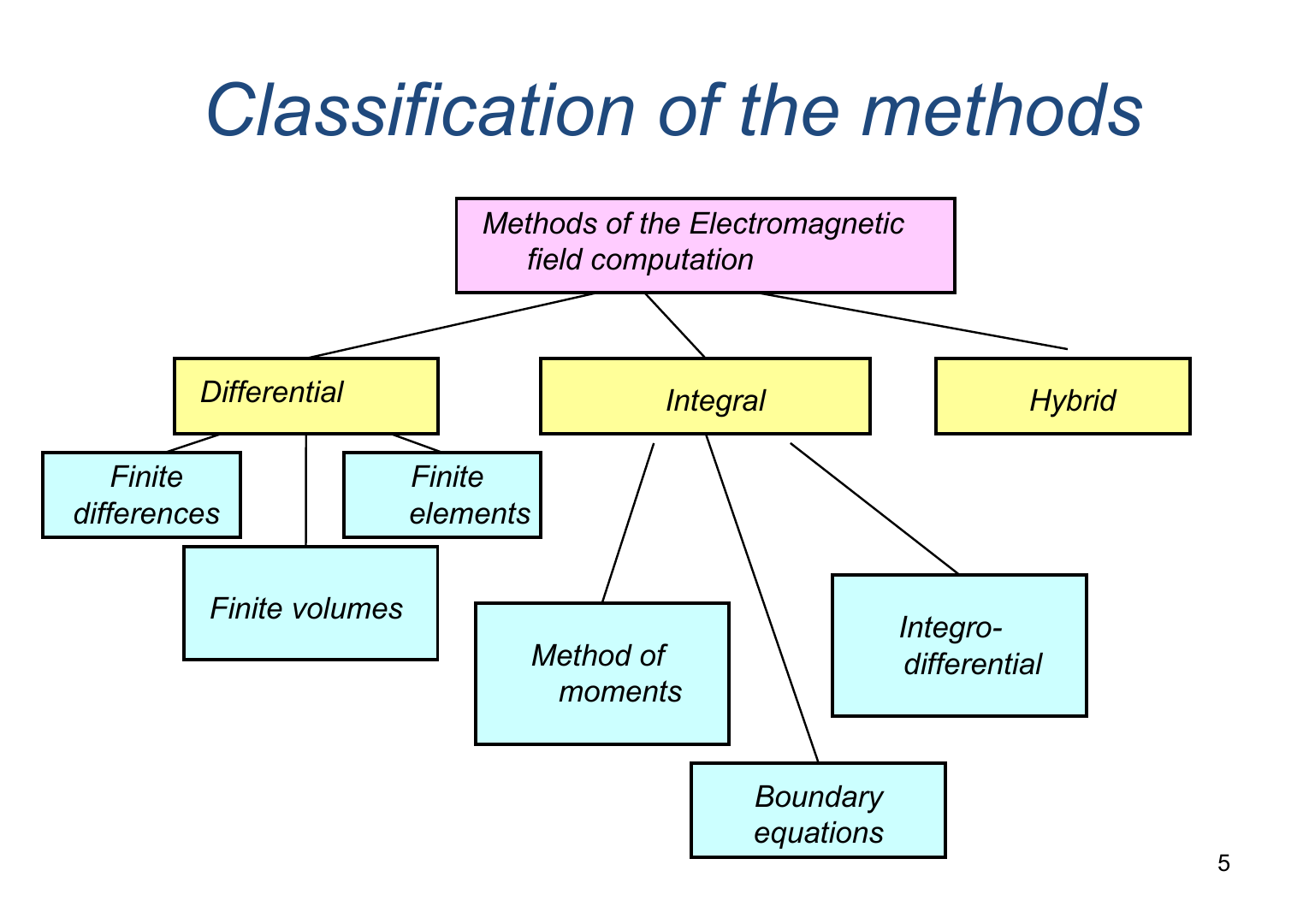
• Finite difference – метод сеток (метод конечных разностей)

• Finite elements – метод конечных элементов (используется в Quickfield)

• Finite volumes – метод конечных объемов

• Method of moments (method of spatial equations) – метод моментов

• Boundary equations – метод граничных уравнений

• Integro-differential – интегрально-дифференциальный метод

Hybrid method combines several methods (Boundary equations+ Finite elements)

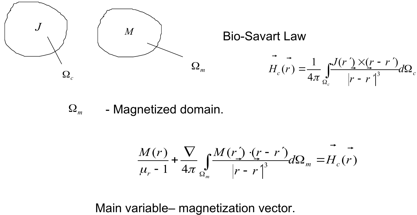
28. Method of moments

This method is quite simple but is not very accurate. It is usually applied to solving magnetic problems. The basis of this method is a system of a several basic equations.

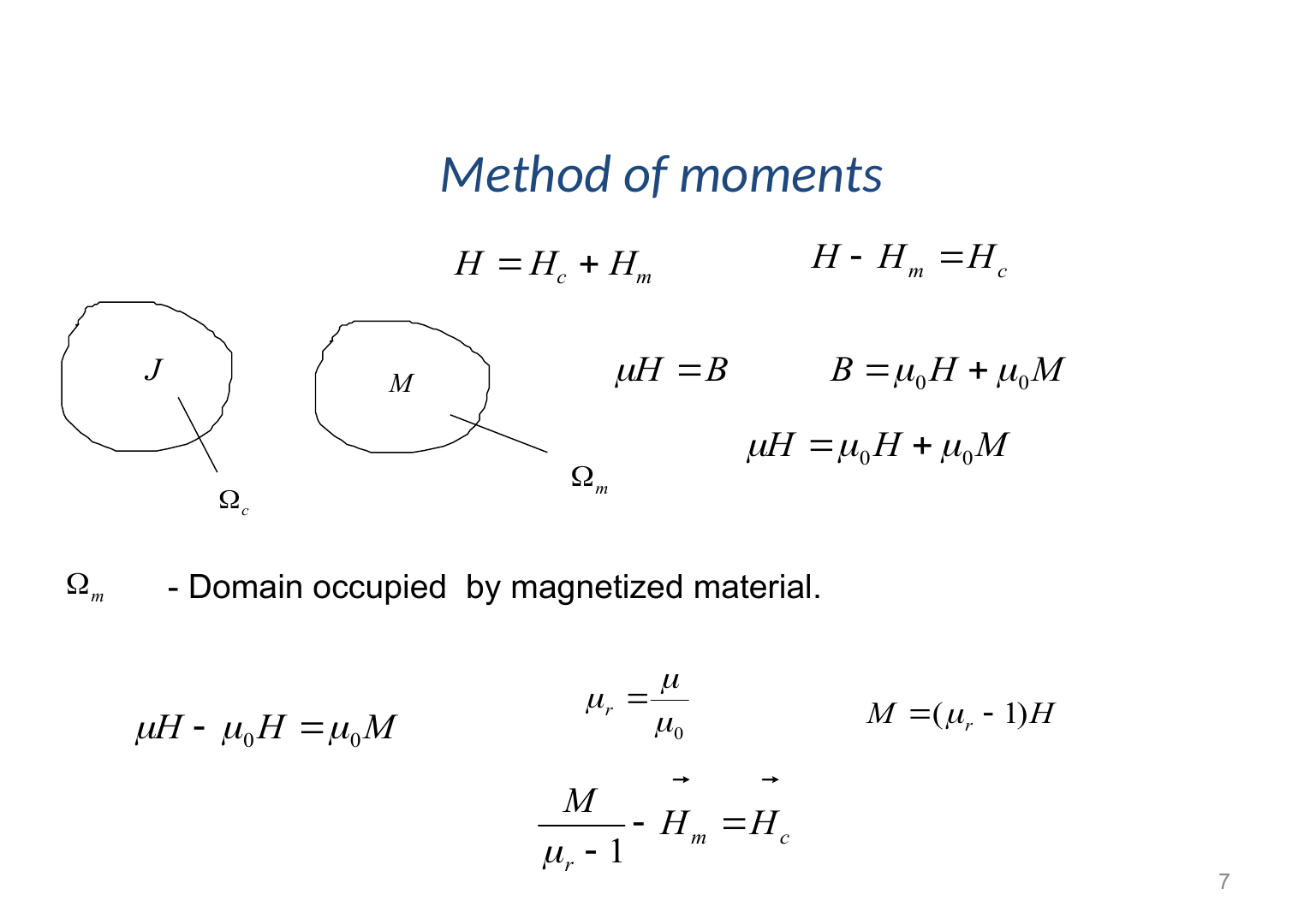
Hm – magnetic field induced by the magnetized object

Hc – magnetic field induced by the current (may be calculated independently on solving the general problem by Biot-Savart Law or another)

МЮr -relative magnetic permeability

M – magnetization

МЮо – magnetic permeability in vacuum

Here and then we will assume, that we work inside isotropic medium.

The general system may consist of volume which if field with magnetize material (область M). may be ferromagnetic (H=102–103) or a material with smaller magnetic permeability. Another part of the volume is the field with the primary sources (область J) (usually currents, but also it may be permanent magnet)

These two volumes are surrounded by air or vacuum. In principle the domain may be infinitely big (tend to infinity). Method of moments hasn’t boundaries, so in this case it is more accurate, than other methods.

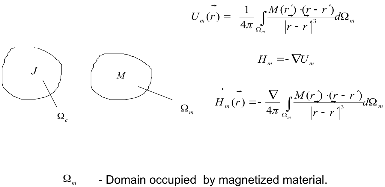
Um – reduced magnetic potential

The first relation is some kind of the Coulomb Law for the magnetic field. So, we use magnetization instead of charges.

We have changed a variable. Now is not field intensity the unknown value, but magnetization.