Discretization of the problem domain (Дискретизация проблемной области)

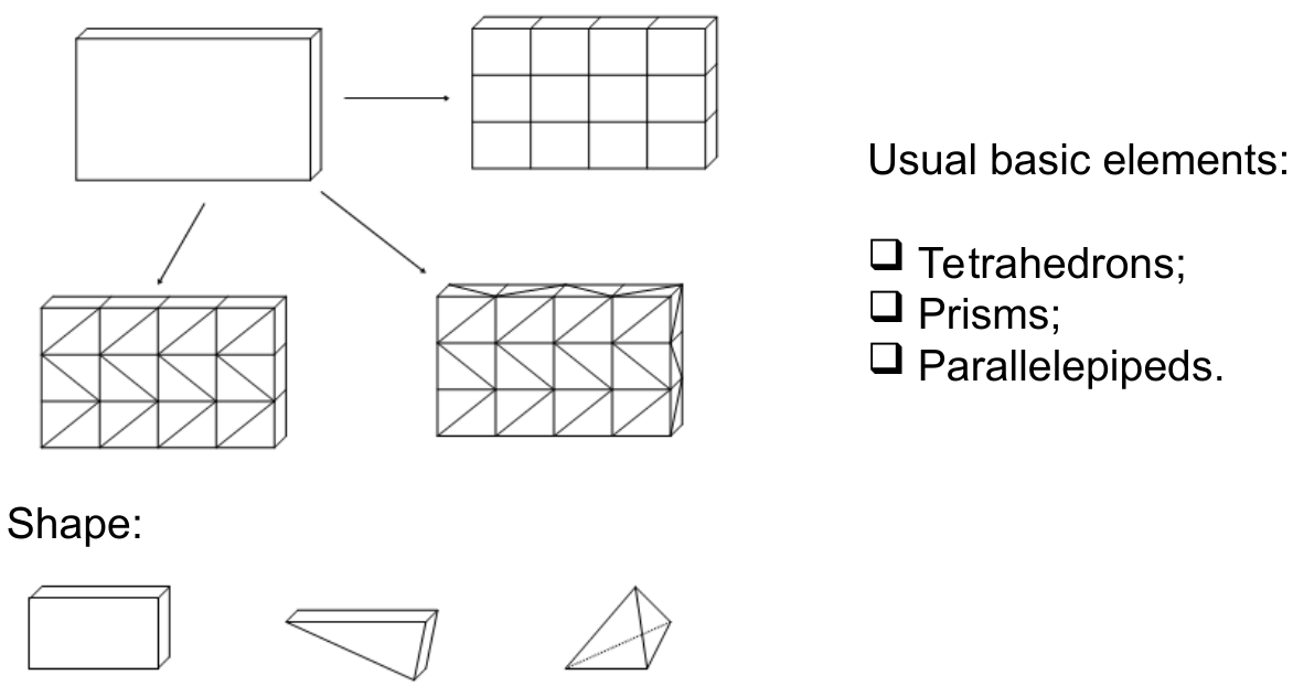
We should split the brick into basic elements (tetrahedrons (тетраэдры), prisms or parallelepipeds)

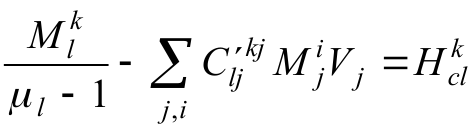
Algebraic equation system (Алгебраическая система уравнений)

• The magnetization of each element is considered constant (the simplest approach). More complex approximation schemes are not used.

• To form a system of equations the method is collocations is used (we must choose some central point inside the element and the magnetic field which induced by all parts of the magnetic system is calculated just for this central point. And then, it’s assumed, that everywhere inside the element the magnetic field intensity has the same value)

29. Basic principles of the finite element method.

Main steps:

1. Problem formulation – problem domain, equation, boundary conditions, material properties.

2. Discretization of the problem domain.

3. Approximation of the unknown function.

4. Approximation of the solved equation and the boundary conditions.

5. Solution of the algebraic equation system (generally – nonlinear).

6. Post-processing (постобработка).

Discretization (Дискретизация)

The element type choice

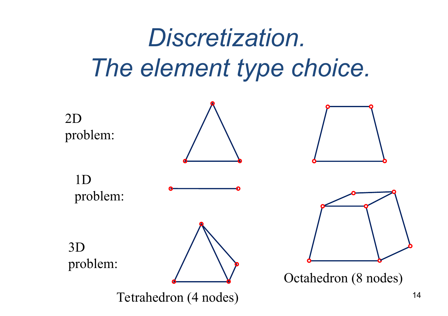
Node – узел (точка, вершина)

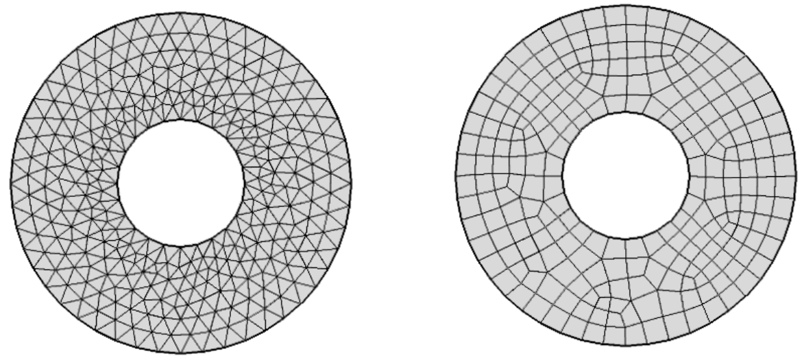
Examples of the mesh (triangles and quadrangles)

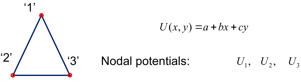
Linear approximation

узловые бля

The number of free parameters is the same!

In principle we can express coefficients a, b, c in terms of the nodal potentials U₁, U₂, U₃

In linear approximation the vertices are the same with the nodal.

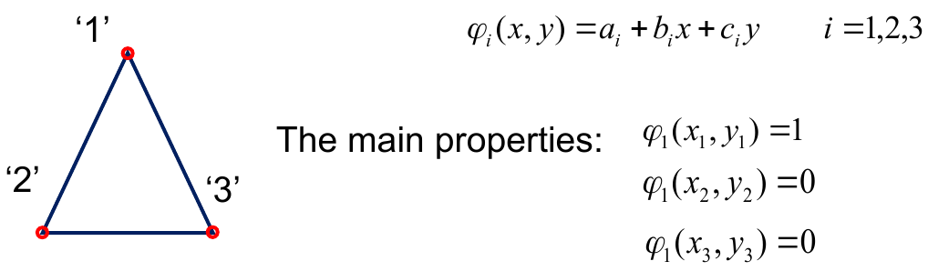
30. Finite functions (Ограниченная функция – отлична от нуля только в пределах треугольника)

Finite function inside the triangle may have different dependences. Everything depends on the value of the nodal potential.

There are three very special finite function:

• F inite function associated with the first node:

Similar relations are valid for 2 other finite functions.

Finite functions for triangles = simplex coordinates (coordinates – because every point inside the triangle may be describe by certain value of finite functions, that is why the behavior of these functions is similar to coordinates).

Simplex coordinates

Two-dimensional simplex coordinates:

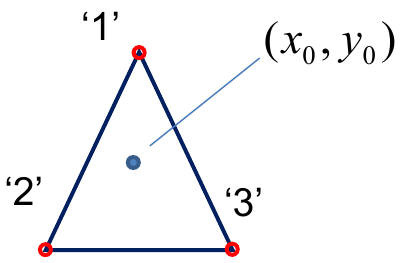
Another definition of the point position is a set of simplex coordinates

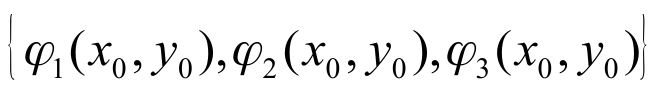
Really only 2 of 3 simplex coordinates are independent:

General relation for the simplex coordinates:

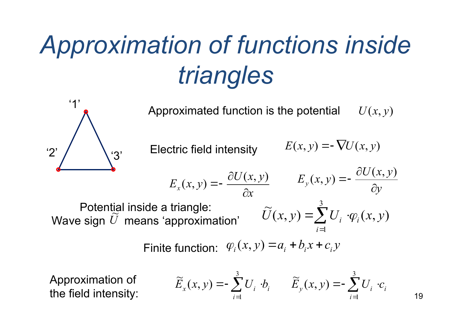
Approximation of functions inside triangles (Аппроксимация функций внутри треугольника)

Approximated function is the potential: U(x, y)

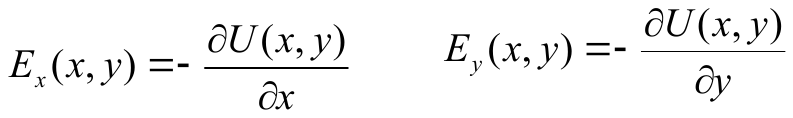
Electric field intensity

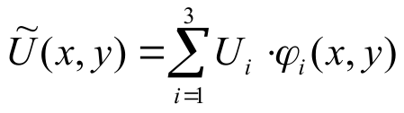
Potential inside a triangle (Wave sign means ‘approximation’):

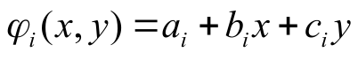
Finite function:

Approximation of the field intensity:

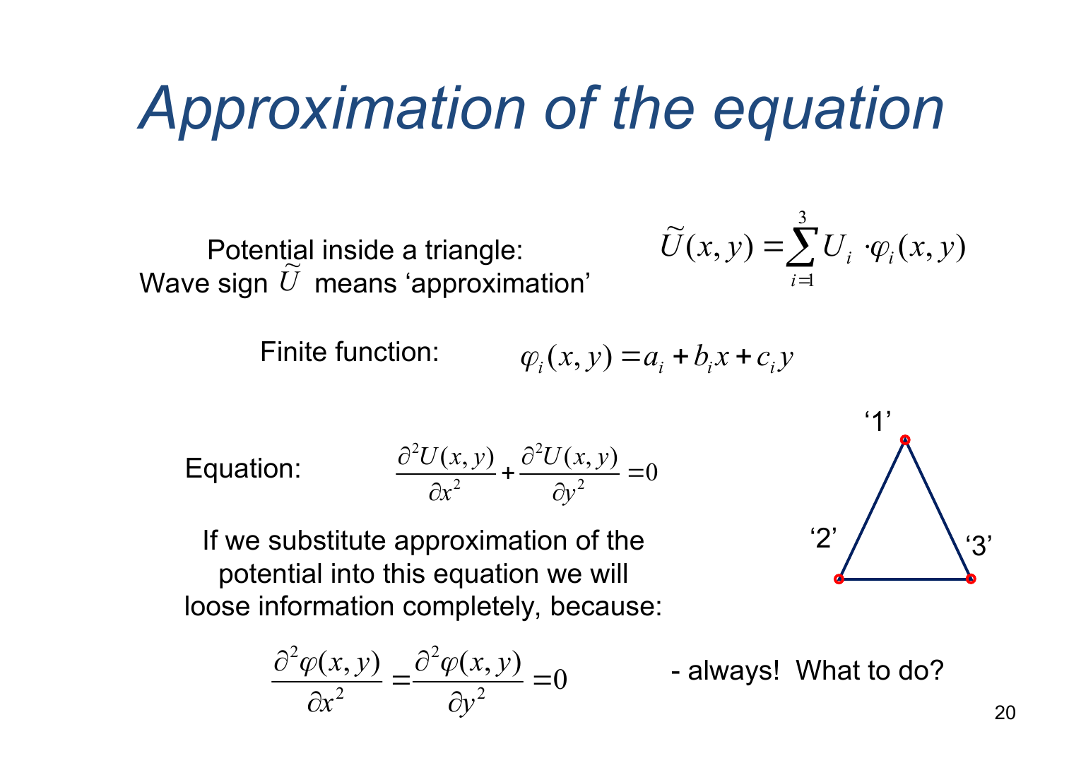
Approximation of the equation (Аппроксимация уравнения)

Potential inside a triangle (Wave sign means ‘approximation’):

Finite function:

Equation:

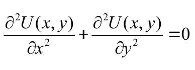
If we substitute approximation of the potential into this equation we will lose information completely, because

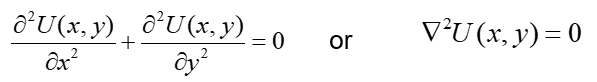
31. Weighted residual method (метод взвешенных невязок)

This method is used to solve different kinds of problems and the idea behind this method is non-trivial. Let’s look to the initial equation:

Let’s choose some arbitrary (произвольную) function ψ(x,y) (можем выбрать некоторую произвольную функцию, которую в будущем назовём взвешенной (weighting) функцией). Evidently, if right initial equation is equal to zero, so the product of this Laplace operator and weighting function will be equal to zero.

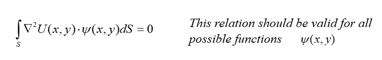
Now let's integrate this product over the area s (this s corresponds to the whole problem domain)

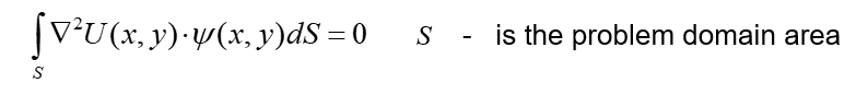
Also, it is necessary to remember, we are talking about finite element method and all finite functions and consequently these weighted functions also will be limited by certain element, they will be equal zero outside the considered element and will be non-zero inside them. That’s why the first glance (взгляд) this integral is very complicated it should be integrate over the wide area, but in the practice it should integrate always in very small area, which is restricted by considered elements.

To choose correctly the weight function we use Galerkin method

This is an initial equation and that is true only because the Laplacian of potential is equal to zero. Evidently, the Laplacian of such approximation not necessary will be equal to zero it may differ from zero, that’s why the integral from the product of Laplacian weighting function and after integration will give us so called ‘weighted residual’ – R:

So, the idea of the Galerkin method – it is the special choice of the weighting functions:

• to use the weighted residual method;

• to use approximation functions for weighting:

• to set residuals to zero; R_j=0

• to apply integration-by-parts procedure to the integral (weak formulation)

Let’s assume that the weighting function is the same of the finite function, which corresponds just to this triangle, of course, there are three different functions, so for every triangle we should use three weighting functions. The second assumption, set residuals to zero, evidently we can choose approximation of the potential in such a way the residual will be really equal to zero, not because the Laplacian of the potential is equal to zero, but because the product of this potential and the weighting function after integration will give zero. And now let’s apply integration-by-parts procedure to the integral.

Indeed, if we shall directly calculate this integral using approximation of the potential, we can get exact zero (zero will be equal to zero), so to avoid this difficulty it is possible to use some mathematic transformation, which is called integration-by-part. Очень важная часть метода Галеркина заключается в том, что прямолинейное вычисление интеграла такого вида даст нам нулевой ответ только потому, что вторая производная от полинома первого порядка всегда равна нулю, и таким образом мы не сможем найти решение. Для того, чтобы преодолеть эту сложность в методе Галеркина предполагается провести идентичное преобразование – интегрирование по частям.