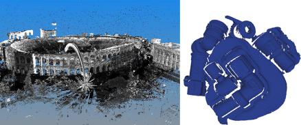
Fig. 6.8 Example of large scan acquisition (left) and scene with multiple mechanical objects (right)

is proposed that creates a global model description using an oriented point pair feature and matches it using a fast voting scheme. This fast voting scheme, similar to the Generalized Hough Transform, is used to optimize the model pose in a locally reduced search space. This space is parametrized in terms of points on the model and rotation around the surface normals.

6.3.3 Deformable Registration

While rigidity in the aligning transformation is a largely applicable constraint, it is too restrictive in some cases. Imagine indeed that the object that has to be registered is not rigid but deformable. Deformable registration has two main issues: the computation of stable correspondences and the use of an appropriate deformation model. Note that the need for registration of articulated or deformable objects has recently increased due to the availability of real-time range scanners [21, 22, 51, 58]. Roughly speaking, we can emphasize two classes of deformable registration methods: (i) methods based on general optimization techniques, and (ii) probabilistic methods.

Methods Based on General Optimization Techniques The general formulation of deformable registration is more involved than the rigid case and it is more difficult to solve in closed-form. Advanced optimization techniques are used instead. The advantage of using general optimization techniques consists of jointly computing the estimation of correspondences and the deformable parameters [21, 22, 24, 51]. Moreover, other unknowns can be used to model further information like the overlapping area, the reliability of correspondences, the smoothness constraint and so on [51]. Examples of transformation models which have been introduced for surface deformations are (i) affine transforms applied to nodes uniformly sampled from the range images [51], (ii) rigid transforms on patches automatically extracted from

the surface [21], (iii) Thin-Plate Splines (TPS) [24, 76], or (iv) linear blend skinning model (LBS) [22]. The error function can be optimized by the Levenberg-Marquardt Algorithm [51], GraphCuts [21], or Expectation-Maximization (EM) [22, 24, 61]. In [42] deformable registration is solved by alternating between correspondence and deformation optimization. Assuming approximately isometric deformations, robust correspondences are generated using a pruning mechanism based on geodesic consistency.

Deformable alignment to account for errors in the point clouds obtained by scanning a rigid object is proposed in [12, 13]. Also, in this case, the authors use TPS to represent the deformable warp between a pair of views, that they estimate through hierarchical ICP [76].

Probabilistic Methods Using probabilistic methods the uncertainty on the correct surface transformation can be addressed by adopting maximum likelihood estimation [2, 28, 41, 46, 61, 96]. Probabilistic approaches are based on modeling each of the point sets by a kernel density function [93]. The dissimilarity among such densities is computed by introducing appropriate distance functions. Registration is carried out without explicitly establishing correspondences. Indeed, the algorithm registers two meshes by optimizing a joint probabilistic model over all point-to-point correspondences between them [2]. In [46], the authors propose a correlation-based approach [93] to point set registration by representing the point sets as Gaussian Mixture Models. A closed-form solution for the L2 norm distance between two Gaussian mixtures makes fast computation possible. In [96], registration is carried out simultaneously for several 3D range datasets. The method proposes an information-theoretic approach based on the Jensen-Shannon divergence measure. In [61], deformable registration is treated as a Maximum Likelihood estimation problem by introducing the Coherent Point Drift paradigm. Smoothness constraints are introduced based on the assumption that points close to one another tend to move coherently over the velocity field. The proposed energy function is minimized with the EM algorithm. A similar approach has been proposed in [28] to track the full hand motion. A stereo set-up is employed to estimate the 3D surface. To improve the estimation of the hand pose, 2D motion (i.e., optical flow) is combined with 3D information. A well defined hand model is employed to deal with articulated structures and deformations. Also in this case the standard ICP algorithm has been extended to its probabilistic version according to the EMICP approach. This approach has been further extended in [41] where the so called Expectation Conditional Maximization paradigm is introduced. A formal demonstration is proposed to show that it is convenient to replace the standard M-step by three conditional maximization steps, or CM-steps, while preserving the convergence properties of EM. Experiments are reported for both hand and body tracking.