
- •Preface
- •Biological Vision Systems
- •Visual Representations from Paintings to Photographs
- •Computer Vision
- •The Limitations of Standard 2D Images
- •3D Imaging, Analysis and Applications
- •Book Objective and Content
- •Acknowledgements
- •Contents
- •Contributors
- •2.1 Introduction
- •Chapter Outline
- •2.2 An Overview of Passive 3D Imaging Systems
- •2.2.1 Multiple View Approaches
- •2.2.2 Single View Approaches
- •2.3 Camera Modeling
- •2.3.1 Homogeneous Coordinates
- •2.3.2 Perspective Projection Camera Model
- •2.3.2.1 Camera Modeling: The Coordinate Transformation
- •2.3.2.2 Camera Modeling: Perspective Projection
- •2.3.2.3 Camera Modeling: Image Sampling
- •2.3.2.4 Camera Modeling: Concatenating the Projective Mappings
- •2.3.3 Radial Distortion
- •2.4 Camera Calibration
- •2.4.1 Estimation of a Scene-to-Image Planar Homography
- •2.4.2 Basic Calibration
- •2.4.3 Refined Calibration
- •2.4.4 Calibration of a Stereo Rig
- •2.5 Two-View Geometry
- •2.5.1 Epipolar Geometry
- •2.5.2 Essential and Fundamental Matrices
- •2.5.3 The Fundamental Matrix for Pure Translation
- •2.5.4 Computation of the Fundamental Matrix
- •2.5.5 Two Views Separated by a Pure Rotation
- •2.5.6 Two Views of a Planar Scene
- •2.6 Rectification
- •2.6.1 Rectification with Calibration Information
- •2.6.2 Rectification Without Calibration Information
- •2.7 Finding Correspondences
- •2.7.1 Correlation-Based Methods
- •2.7.2 Feature-Based Methods
- •2.8 3D Reconstruction
- •2.8.1 Stereo
- •2.8.1.1 Dense Stereo Matching
- •2.8.1.2 Triangulation
- •2.8.2 Structure from Motion
- •2.9 Passive Multiple-View 3D Imaging Systems
- •2.9.1 Stereo Cameras
- •2.9.2 3D Modeling
- •2.9.3 Mobile Robot Localization and Mapping
- •2.10 Passive Versus Active 3D Imaging Systems
- •2.11 Concluding Remarks
- •2.12 Further Reading
- •2.13 Questions
- •2.14 Exercises
- •References
- •3.1 Introduction
- •3.1.1 Historical Context
- •3.1.2 Basic Measurement Principles
- •3.1.3 Active Triangulation-Based Methods
- •3.1.4 Chapter Outline
- •3.2 Spot Scanners
- •3.2.1 Spot Position Detection
- •3.3 Stripe Scanners
- •3.3.1 Camera Model
- •3.3.2 Sheet-of-Light Projector Model
- •3.3.3 Triangulation for Stripe Scanners
- •3.4 Area-Based Structured Light Systems
- •3.4.1 Gray Code Methods
- •3.4.1.1 Decoding of Binary Fringe-Based Codes
- •3.4.1.2 Advantage of the Gray Code
- •3.4.2 Phase Shift Methods
- •3.4.2.1 Removing the Phase Ambiguity
- •3.4.3 Triangulation for a Structured Light System
- •3.5 System Calibration
- •3.6 Measurement Uncertainty
- •3.6.1 Uncertainty Related to the Phase Shift Algorithm
- •3.6.2 Uncertainty Related to Intrinsic Parameters
- •3.6.3 Uncertainty Related to Extrinsic Parameters
- •3.6.4 Uncertainty as a Design Tool
- •3.7 Experimental Characterization of 3D Imaging Systems
- •3.7.1 Low-Level Characterization
- •3.7.2 System-Level Characterization
- •3.7.3 Characterization of Errors Caused by Surface Properties
- •3.7.4 Application-Based Characterization
- •3.8 Selected Advanced Topics
- •3.8.1 Thin Lens Equation
- •3.8.2 Depth of Field
- •3.8.3 Scheimpflug Condition
- •3.8.4 Speckle and Uncertainty
- •3.8.5 Laser Depth of Field
- •3.8.6 Lateral Resolution
- •3.9 Research Challenges
- •3.10 Concluding Remarks
- •3.11 Further Reading
- •3.12 Questions
- •3.13 Exercises
- •References
- •4.1 Introduction
- •Chapter Outline
- •4.2 Representation of 3D Data
- •4.2.1 Raw Data
- •4.2.1.1 Point Cloud
- •4.2.1.2 Structured Point Cloud
- •4.2.1.3 Depth Maps and Range Images
- •4.2.1.4 Needle map
- •4.2.1.5 Polygon Soup
- •4.2.2 Surface Representations
- •4.2.2.1 Triangular Mesh
- •4.2.2.2 Quadrilateral Mesh
- •4.2.2.3 Subdivision Surfaces
- •4.2.2.4 Morphable Model
- •4.2.2.5 Implicit Surface
- •4.2.2.6 Parametric Surface
- •4.2.2.7 Comparison of Surface Representations
- •4.2.3 Solid-Based Representations
- •4.2.3.1 Voxels
- •4.2.3.3 Binary Space Partitioning
- •4.2.3.4 Constructive Solid Geometry
- •4.2.3.5 Boundary Representations
- •4.2.4 Summary of Solid-Based Representations
- •4.3 Polygon Meshes
- •4.3.1 Mesh Storage
- •4.3.2 Mesh Data Structures
- •4.3.2.1 Halfedge Structure
- •4.4 Subdivision Surfaces
- •4.4.1 Doo-Sabin Scheme
- •4.4.2 Catmull-Clark Scheme
- •4.4.3 Loop Scheme
- •4.5 Local Differential Properties
- •4.5.1 Surface Normals
- •4.5.2 Differential Coordinates and the Mesh Laplacian
- •4.6 Compression and Levels of Detail
- •4.6.1 Mesh Simplification
- •4.6.1.1 Edge Collapse
- •4.6.1.2 Quadric Error Metric
- •4.6.2 QEM Simplification Summary
- •4.6.3 Surface Simplification Results
- •4.7 Visualization
- •4.8 Research Challenges
- •4.9 Concluding Remarks
- •4.10 Further Reading
- •4.11 Questions
- •4.12 Exercises
- •References
- •1.1 Introduction
- •Chapter Outline
- •1.2 A Historical Perspective on 3D Imaging
- •1.2.1 Image Formation and Image Capture
- •1.2.2 Binocular Perception of Depth
- •1.2.3 Stereoscopic Displays
- •1.3 The Development of Computer Vision
- •1.3.1 Further Reading in Computer Vision
- •1.4 Acquisition Techniques for 3D Imaging
- •1.4.1 Passive 3D Imaging
- •1.4.2 Active 3D Imaging
- •1.4.3 Passive Stereo Versus Active Stereo Imaging
- •1.5 Twelve Milestones in 3D Imaging and Shape Analysis
- •1.5.1 Active 3D Imaging: An Early Optical Triangulation System
- •1.5.2 Passive 3D Imaging: An Early Stereo System
- •1.5.3 Passive 3D Imaging: The Essential Matrix
- •1.5.4 Model Fitting: The RANSAC Approach to Feature Correspondence Analysis
- •1.5.5 Active 3D Imaging: Advances in Scanning Geometries
- •1.5.6 3D Registration: Rigid Transformation Estimation from 3D Correspondences
- •1.5.7 3D Registration: Iterative Closest Points
- •1.5.9 3D Local Shape Descriptors: Spin Images
- •1.5.10 Passive 3D Imaging: Flexible Camera Calibration
- •1.5.11 3D Shape Matching: Heat Kernel Signatures
- •1.6 Applications of 3D Imaging
- •1.7 Book Outline
- •1.7.1 Part I: 3D Imaging and Shape Representation
- •1.7.2 Part II: 3D Shape Analysis and Processing
- •1.7.3 Part III: 3D Imaging Applications
- •References
- •5.1 Introduction
- •5.1.1 Applications
- •5.1.2 Chapter Outline
- •5.2 Mathematical Background
- •5.2.1 Differential Geometry
- •5.2.2 Curvature of Two-Dimensional Surfaces
- •5.2.3 Discrete Differential Geometry
- •5.2.4 Diffusion Geometry
- •5.2.5 Discrete Diffusion Geometry
- •5.3 Feature Detectors
- •5.3.1 A Taxonomy
- •5.3.2 Harris 3D
- •5.3.3 Mesh DOG
- •5.3.4 Salient Features
- •5.3.5 Heat Kernel Features
- •5.3.6 Topological Features
- •5.3.7 Maximally Stable Components
- •5.3.8 Benchmarks
- •5.4 Feature Descriptors
- •5.4.1 A Taxonomy
- •5.4.2 Curvature-Based Descriptors (HK and SC)
- •5.4.3 Spin Images
- •5.4.4 Shape Context
- •5.4.5 Integral Volume Descriptor
- •5.4.6 Mesh Histogram of Gradients (HOG)
- •5.4.7 Heat Kernel Signature (HKS)
- •5.4.8 Scale-Invariant Heat Kernel Signature (SI-HKS)
- •5.4.9 Color Heat Kernel Signature (CHKS)
- •5.4.10 Volumetric Heat Kernel Signature (VHKS)
- •5.5 Research Challenges
- •5.6 Conclusions
- •5.7 Further Reading
- •5.8 Questions
- •5.9 Exercises
- •References
- •6.1 Introduction
- •Chapter Outline
- •6.2 Registration of Two Views
- •6.2.1 Problem Statement
- •6.2.2 The Iterative Closest Points (ICP) Algorithm
- •6.2.3 ICP Extensions
- •6.2.3.1 Techniques for Pre-alignment
- •Global Approaches
- •Local Approaches
- •6.2.3.2 Techniques for Improving Speed
- •Subsampling
- •Closest Point Computation
- •Distance Formulation
- •6.2.3.3 Techniques for Improving Accuracy
- •Outlier Rejection
- •Additional Information
- •Probabilistic Methods
- •6.3 Advanced Techniques
- •6.3.1 Registration of More than Two Views
- •Reducing Error Accumulation
- •Automating Registration
- •6.3.2 Registration in Cluttered Scenes
- •Point Signatures
- •Matching Methods
- •6.3.3 Deformable Registration
- •Methods Based on General Optimization Techniques
- •Probabilistic Methods
- •6.3.4 Machine Learning Techniques
- •Improving the Matching
- •Object Detection
- •6.4 Quantitative Performance Evaluation
- •6.5 Case Study 1: Pairwise Alignment with Outlier Rejection
- •6.6 Case Study 2: ICP with Levenberg-Marquardt
- •6.6.1 The LM-ICP Method
- •6.6.2 Computing the Derivatives
- •6.6.3 The Case of Quaternions
- •6.6.4 Summary of the LM-ICP Algorithm
- •6.6.5 Results and Discussion
- •6.7 Case Study 3: Deformable ICP with Levenberg-Marquardt
- •6.7.1 Surface Representation
- •6.7.2 Cost Function
- •Data Term: Global Surface Attraction
- •Data Term: Boundary Attraction
- •Penalty Term: Spatial Smoothness
- •Penalty Term: Temporal Smoothness
- •6.7.3 Minimization Procedure
- •6.7.4 Summary of the Algorithm
- •6.7.5 Experiments
- •6.8 Research Challenges
- •6.9 Concluding Remarks
- •6.10 Further Reading
- •6.11 Questions
- •6.12 Exercises
- •References
- •7.1 Introduction
- •7.1.1 Retrieval and Recognition Evaluation
- •7.1.2 Chapter Outline
- •7.2 Literature Review
- •7.3 3D Shape Retrieval Techniques
- •7.3.1 Depth-Buffer Descriptor
- •7.3.1.1 Computing the 2D Projections
- •7.3.1.2 Obtaining the Feature Vector
- •7.3.1.3 Evaluation
- •7.3.1.4 Complexity Analysis
- •7.3.2 Spin Images for Object Recognition
- •7.3.2.1 Matching
- •7.3.2.2 Evaluation
- •7.3.2.3 Complexity Analysis
- •7.3.3 Salient Spectral Geometric Features
- •7.3.3.1 Feature Points Detection
- •7.3.3.2 Local Descriptors
- •7.3.3.3 Shape Matching
- •7.3.3.4 Evaluation
- •7.3.3.5 Complexity Analysis
- •7.3.4 Heat Kernel Signatures
- •7.3.4.1 Evaluation
- •7.3.4.2 Complexity Analysis
- •7.4 Research Challenges
- •7.5 Concluding Remarks
- •7.6 Further Reading
- •7.7 Questions
- •7.8 Exercises
- •References
- •8.1 Introduction
- •Chapter Outline
- •8.2 3D Face Scan Representation and Visualization
- •8.3 3D Face Datasets
- •8.3.1 FRGC v2 3D Face Dataset
- •8.3.2 The Bosphorus Dataset
- •8.4 3D Face Recognition Evaluation
- •8.4.1 Face Verification
- •8.4.2 Face Identification
- •8.5 Processing Stages in 3D Face Recognition
- •8.5.1 Face Detection and Segmentation
- •8.5.2 Removal of Spikes
- •8.5.3 Filling of Holes and Missing Data
- •8.5.4 Removal of Noise
- •8.5.5 Fiducial Point Localization and Pose Correction
- •8.5.6 Spatial Resampling
- •8.5.7 Feature Extraction on Facial Surfaces
- •8.5.8 Classifiers for 3D Face Matching
- •8.6 ICP-Based 3D Face Recognition
- •8.6.1 ICP Outline
- •8.6.2 A Critical Discussion of ICP
- •8.6.3 A Typical ICP-Based 3D Face Recognition Implementation
- •8.6.4 ICP Variants and Other Surface Registration Approaches
- •8.7 PCA-Based 3D Face Recognition
- •8.7.1 PCA System Training
- •8.7.2 PCA Training Using Singular Value Decomposition
- •8.7.3 PCA Testing
- •8.7.4 PCA Performance
- •8.8 LDA-Based 3D Face Recognition
- •8.8.1 Two-Class LDA
- •8.8.2 LDA with More than Two Classes
- •8.8.3 LDA in High Dimensional 3D Face Spaces
- •8.8.4 LDA Performance
- •8.9 Normals and Curvature in 3D Face Recognition
- •8.9.1 Computing Curvature on a 3D Face Scan
- •8.10 Recent Techniques in 3D Face Recognition
- •8.10.1 3D Face Recognition Using Annotated Face Models (AFM)
- •8.10.2 Local Feature-Based 3D Face Recognition
- •8.10.2.1 Keypoint Detection and Local Feature Matching
- •8.10.2.2 Other Local Feature-Based Methods
- •8.10.3 Expression Modeling for Invariant 3D Face Recognition
- •8.10.3.1 Other Expression Modeling Approaches
- •8.11 Research Challenges
- •8.12 Concluding Remarks
- •8.13 Further Reading
- •8.14 Questions
- •8.15 Exercises
- •References
- •9.1 Introduction
- •Chapter Outline
- •9.2 DEM Generation from Stereoscopic Imagery
- •9.2.1 Stereoscopic DEM Generation: Literature Review
- •9.2.2 Accuracy Evaluation of DEMs
- •9.2.3 An Example of DEM Generation from SPOT-5 Imagery
- •9.3 DEM Generation from InSAR
- •9.3.1 Techniques for DEM Generation from InSAR
- •9.3.1.1 Basic Principle of InSAR in Elevation Measurement
- •9.3.1.2 Processing Stages of DEM Generation from InSAR
- •The Branch-Cut Method of Phase Unwrapping
- •The Least Squares (LS) Method of Phase Unwrapping
- •9.3.2 Accuracy Analysis of DEMs Generated from InSAR
- •9.3.3 Examples of DEM Generation from InSAR
- •9.4 DEM Generation from LIDAR
- •9.4.1 LIDAR Data Acquisition
- •9.4.2 Accuracy, Error Types and Countermeasures
- •9.4.3 LIDAR Interpolation
- •9.4.4 LIDAR Filtering
- •9.4.5 DTM from Statistical Properties of the Point Cloud
- •9.5 Research Challenges
- •9.6 Concluding Remarks
- •9.7 Further Reading
- •9.8 Questions
- •9.9 Exercises
- •References
- •10.1 Introduction
- •10.1.1 Allometric Modeling of Biomass
- •10.1.2 Chapter Outline
- •10.2 Aerial Photo Mensuration
- •10.2.1 Principles of Aerial Photogrammetry
- •10.2.1.1 Geometric Basis of Photogrammetric Measurement
- •10.2.1.2 Ground Control and Direct Georeferencing
- •10.2.2 Tree Height Measurement Using Forest Photogrammetry
- •10.2.2.2 Automated Methods in Forest Photogrammetry
- •10.3 Airborne Laser Scanning
- •10.3.1 Principles of Airborne Laser Scanning
- •10.3.1.1 Lidar-Based Measurement of Terrain and Canopy Surfaces
- •10.3.2 Individual Tree-Level Measurement Using Lidar
- •10.3.2.1 Automated Individual Tree Measurement Using Lidar
- •10.3.3 Area-Based Approach to Estimating Biomass with Lidar
- •10.4 Future Developments
- •10.5 Concluding Remarks
- •10.6 Further Reading
- •10.7 Questions
- •References
- •11.1 Introduction
- •Chapter Outline
- •11.2 Volumetric Data Acquisition
- •11.2.1 Computed Tomography
- •11.2.1.1 Characteristics of 3D CT Data
- •11.2.2 Positron Emission Tomography (PET)
- •11.2.2.1 Characteristics of 3D PET Data
- •Relaxation
- •11.2.3.1 Characteristics of the 3D MRI Data
- •Image Quality and Artifacts
- •11.2.4 Summary
- •11.3 Surface Extraction and Volumetric Visualization
- •11.3.1 Surface Extraction
- •Example: Curvatures and Geometric Tools
- •11.3.2 Volume Rendering
- •11.3.3 Summary
- •11.4 Volumetric Image Registration
- •11.4.1 A Hierarchy of Transformations
- •11.4.1.1 Rigid Body Transformation
- •11.4.1.2 Similarity Transformations and Anisotropic Scaling
- •11.4.1.3 Affine Transformations
- •11.4.1.4 Perspective Transformations
- •11.4.1.5 Non-rigid Transformations
- •11.4.2 Points and Features Used for the Registration
- •11.4.2.1 Landmark Features
- •11.4.2.2 Surface-Based Registration
- •11.4.2.3 Intensity-Based Registration
- •11.4.3 Registration Optimization
- •11.4.3.1 Estimation of Registration Errors
- •11.4.4 Summary
- •11.5 Segmentation
- •11.5.1 Semi-automatic Methods
- •11.5.1.1 Thresholding
- •11.5.1.2 Region Growing
- •11.5.1.3 Deformable Models
- •Snakes
- •Balloons
- •11.5.2 Fully Automatic Methods
- •11.5.2.1 Atlas-Based Segmentation
- •11.5.2.2 Statistical Shape Modeling and Analysis
- •11.5.3 Summary
- •11.6 Diffusion Imaging: An Illustration of a Full Pipeline
- •11.6.1 From Scalar Images to Tensors
- •11.6.2 From Tensor Image to Information
- •11.6.3 Summary
- •11.7 Applications
- •11.7.1 Diagnosis and Morphometry
- •11.7.2 Simulation and Training
- •11.7.3 Surgical Planning and Guidance
- •11.7.4 Summary
- •11.8 Concluding Remarks
- •11.9 Research Challenges
- •11.10 Further Reading
- •Data Acquisition
- •Surface Extraction
- •Volume Registration
- •Segmentation
- •Diffusion Imaging
- •Software
- •11.11 Questions
- •11.12 Exercises
- •References
- •Index

5 Feature-Based Methods in 3D Shape Analysis |
207 |
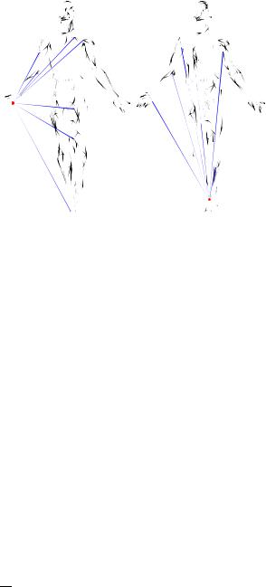
Fig. 5.5 Example of shape context computation. Shown in red is the reference point x, and in blue the rays y − x
Given the coordinates of a point x on the shape, the shape context descriptor is constructed as a histogram of the direction vectors from x to the rest of the points, y − x. Typically, a log-polar histogram is used. The descriptor is applicable to any shape representation in which the point coordinates are explicitly given, such as mesh, point cloud, or volume. Such a descriptor is not deformation-invariant, due to its dependence on the embedding coordinates. An example of shape context computation is shown in Fig. 5.5.
5.4.5 Integral Volume Descriptor
The integral volume descriptor, used in [34], is an extension to 3D shapes of the concept of integral invariants introduced for image description in [54]. Given a solid object Ω with a boundary X = ∂Ω , the descriptor measures volume contained in a ball of fixed radius r ,
Vr (x) = |
dx. |
(5.29) |
|
Br (x)∩Ω |
|
If Br (x) ∩ Ω is simply connected, the volume descriptor can be related to the mean curvature H (x) as Vr (x) = 23π r3 − π4 H r4 + O (r5) [34]. Since the mean curvature is not intrinsic, the descriptor is sensitive to deformations of the shape. Varying the value of r , a multi-scale descriptor can be computed. Numerically, the descriptor is efficiently computed in a voxel representation of the shape, by means of convolution with the ball mask.
208 |
A.M. Bronstein et al. |
5.4.6 Mesh Histogram of Gradients (HOG)
MeshHOG [87] is a shape descriptor emulating SIFT-like image descriptors [51], referred to as histograms of gradients or HOG. The descriptor assumes the shape in mesh representation and in addition to be given some function f defined on the mesh vertices. The function can be either photometric information (texture) or a geometric quantity such as curvature. The descriptor at point x is computed by creating a local histogram of gradients of f in an r -ring neighborhood of x. The gradient f is defined extrinsically as a vector in R3 but projected onto the tangent plane at x which makes it intrinsic. The descriptor support is divided into four polar slices (corresponding to 16 quadrants in SIFT). For each of the slices, a histogram of 8 gradient orientations is computed. The result is a 32-dimensional descriptor vector obtained by concatenating the histogram bins.
The MeshHOG descriptor works with mesh representations and can work with photometric or geometric data or both. It is intrinsic in theory, though the specific implementation in [87] depends on triangulation.
5.4.7 Heat Kernel Signature (HKS)
The heat kernel signature (HKS) was proposed in [81] as an intrinsic descriptor based on the properties of heat diffusion and defined as the diagonal of the heat kernel. Given some fixed time values t1, . . . , tn, for each point x on the shape, the HKS is an n-dimensional descriptor vector
p(x) = kt1 (x, x), . . . , ktn (x, x) . |
(5.30) |
Intuitively, the diagonal values of the heat kernel indicate how much heat remains at a point after certain time (or alternatively, the probability of a random walk to remain at a point if resorting to the probabilistic interpretation of diffusion processes) and is thus related to the “stability” of a point under diffusion process.
The HKS descriptor is intrinsic and thus isometry-invariant, captures local geometric information at multiple scales, is insensitive to topological noise, and is informative (if the Laplace-Beltrami operator of a shape is non-degenerate, then any continuous map that preserves the HKS at every point must be an isometry). Since the HKS can be expressed in the Laplace-Beltrami eigenbasis as
kt (x, x) |
= |
e−t λi φ |
2 |
(x), |
(5.31) |
|
|
i |
|
|
i≥0
it is easily computed across different shape representations for which there is a way to compute the Laplace-Beltrami eigenfunctions and eigenvalues.

5 Feature-Based Methods in 3D Shape Analysis |
209 |
|||||
|
|
|
|
|
|
|
|
|
|
|
|
|
|
Fig. 5.6 Construction of the Scale-Invariant HKS: (a) we show the HKS computed at the same point, for a shape that is scaled by a factor of 11 (blue dashed plot); please notice the log-scale.
(b) The signal ˜ , where the change in scale has been converted into a shifting in time. (c) The h(τ )
first 10 components of |H˜ (ω)| for the two signals; the descriptors computed at the two different scales are virtually identical
5.4.8 Scale-Invariant Heat Kernel Signature (SI-HKS)
A disadvantage of the HKS is its dependence on the global scale of the shape. If X is globally scaled by β, the corresponding HKS is β−2kβ−2t (x, x). In some cases, it is possible to remove this dependence by global normalization of the shape.
A scale-invariant HKS (SI-HKS) based on local normalization was proposed in [20]. Firstly, the heat kernel scale is sampled logarithmically with some basis α, denoted here as k(τ ) = kατ (x, x). In this scale-space, the heat kernel of the scaled shape becomes k (τ ) = a−2k(τ + 2 logα a) (Fig. 5.6a). Secondly, in order to remove the dependence on the multiplicative constant a−2, the logarithm of the signal followed by a derivative w.r.t. the scale variable is taken,
d
dτ
Denoting
˜
k(τ
log k (τ ) = |
|
d |
|
|
−2 log a + log k(τ + 2 logα a) |
|||||||||||
|
|
|
||||||||||||||
dτ |
||||||||||||||||
|
|
|
= |
|
d |
|
|
log k(τ |
+ 2 logα a) |
|
|
|
||||
|
|
|
|
|
|
|
|
|
||||||||
|
|
|
dτ |
|
|
|
||||||||||
|
|
|
|
|
|
|
d |
k(τ + 2 logα a) |
|
|
|
|||||
|
|
|
= |
|
|
dτ |
|
|
|
|||||||
|
|
|
|
|
|
. |
|
|
|
|||||||
|
|
|
|
|
k(τ + 2 logα a) |
|
|
|
||||||||
|
|
d |
k(τ ) |
|
|
|
− |
i≥0 |
λi ατ log αe−λi ατ |
φ2 |
(x) |
|||||
|
|
dτ |
|
|
|
|||||||||||
) = |
|
|
|
= |
|
|
i |
|
, |
|||||||
|
h(τ ) |
|
|
|
|
i≥0 e−λi ατ φi2(x) |
|
|
(5.32)
(5.33)
|
˜ |
|
|
|
|
|
˜ |
(τ ) |
= |
˜ |
+ |
2 log |
α |
|
as a |
|
one thus has a new function k |
which transforms as k |
|
k(τ |
|
a) |
|||||||||||
result of scaling (Fig. 5.6b). Finally, by applying the Fourier transform to |
˜ |
, the |
||||||||||||||
|
|
|
|
|
|
|
|
|
|
|
|
|
|
|
k |
|
shift becomes a complex phase, |
|
˜ |
|
|
= |
˜ |
|
|
|
|
|
|
|
|
||
˜ |
|
= |
|
|
|
|
|
|
|
|
|
|||||
F k |
(ω) |
|
|
K |
|
(ω) |
|
K (ω)e−j ω2 logα a , |
|
|
|
|
(5.34) |

210 |
A.M. Bronstein et al. |
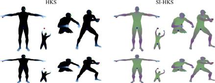
Fig. 5.7 Top: three components of the HKS (left) and the proposed SI-HKS (right), represented as RGB color and shown for different shape transformations (null, isometric deformation+scale, missing part, topological transformation). Bottom: HKS (left) and SI-HKS (right) descriptors at three points of the shape (marked with red, green, and blue). Dashed line shows the null shape descriptor
and taking the absolute value in the Fourier domain (Fig. 5.6c),
˜ |
(ω) |
= |
˜ |
(5.35) |
K |
|
K (ω) , |
produces a scale-invariant descriptor (Fig. 5.7).
5.4.9 Color Heat Kernel Signature (CHKS)
If, in addition, photometric information is available, given in the form of texture α : X → C in some m-dimensional colorspace C (e.g. m = 1 in case of grayscale texture and m = 3 in case of color texture), it is possible to design diffusion processes that take into consideration not only geometric but also photometric information [47, 77]. For this purpose, let us assume the shape X to be a submanifold of some (m + 3)-dimensional manifold E = R3 × C with the Riemannian metric tensor g, embedded by means of a diffeomorphism ξ : X → ξ(X) E . A Riemannian metric on the manifold X induced by the embedding is the pullback metric
(ξ g)(r, s) = g(dξ(r), dξ(s)) for r, s Tx X, where dξ : Tx X → Tξ(x)E is the differential of ξ , and T denotes the tangent space. In coordinate notation, the pullback metric is expressed as (ξ g)μν = gij ∂μξ i ∂ν ξ j , where the indices i, j = 1, . . . , m + 3 denote the embedding coordinates.
The structure of E is to model joint geometric and photometric information. The geometric information is expressed by the embedding coordinates ξg =
(ξ 1, . . . , ξ 3); the photometric information is expressed by the embedding coordinates ξp = (ξ 4, . . . , ξ 3+m) = (α1, . . . , αm). In a simple case when C has a Euclidean structure (for example, the Lab colorspace has a natural Euclidean metric),
the pullback metric boils down to (ξ g)μν