
- •Preface
- •Biological Vision Systems
- •Visual Representations from Paintings to Photographs
- •Computer Vision
- •The Limitations of Standard 2D Images
- •3D Imaging, Analysis and Applications
- •Book Objective and Content
- •Acknowledgements
- •Contents
- •Contributors
- •2.1 Introduction
- •Chapter Outline
- •2.2 An Overview of Passive 3D Imaging Systems
- •2.2.1 Multiple View Approaches
- •2.2.2 Single View Approaches
- •2.3 Camera Modeling
- •2.3.1 Homogeneous Coordinates
- •2.3.2 Perspective Projection Camera Model
- •2.3.2.1 Camera Modeling: The Coordinate Transformation
- •2.3.2.2 Camera Modeling: Perspective Projection
- •2.3.2.3 Camera Modeling: Image Sampling
- •2.3.2.4 Camera Modeling: Concatenating the Projective Mappings
- •2.3.3 Radial Distortion
- •2.4 Camera Calibration
- •2.4.1 Estimation of a Scene-to-Image Planar Homography
- •2.4.2 Basic Calibration
- •2.4.3 Refined Calibration
- •2.4.4 Calibration of a Stereo Rig
- •2.5 Two-View Geometry
- •2.5.1 Epipolar Geometry
- •2.5.2 Essential and Fundamental Matrices
- •2.5.3 The Fundamental Matrix for Pure Translation
- •2.5.4 Computation of the Fundamental Matrix
- •2.5.5 Two Views Separated by a Pure Rotation
- •2.5.6 Two Views of a Planar Scene
- •2.6 Rectification
- •2.6.1 Rectification with Calibration Information
- •2.6.2 Rectification Without Calibration Information
- •2.7 Finding Correspondences
- •2.7.1 Correlation-Based Methods
- •2.7.2 Feature-Based Methods
- •2.8 3D Reconstruction
- •2.8.1 Stereo
- •2.8.1.1 Dense Stereo Matching
- •2.8.1.2 Triangulation
- •2.8.2 Structure from Motion
- •2.9 Passive Multiple-View 3D Imaging Systems
- •2.9.1 Stereo Cameras
- •2.9.2 3D Modeling
- •2.9.3 Mobile Robot Localization and Mapping
- •2.10 Passive Versus Active 3D Imaging Systems
- •2.11 Concluding Remarks
- •2.12 Further Reading
- •2.13 Questions
- •2.14 Exercises
- •References
- •3.1 Introduction
- •3.1.1 Historical Context
- •3.1.2 Basic Measurement Principles
- •3.1.3 Active Triangulation-Based Methods
- •3.1.4 Chapter Outline
- •3.2 Spot Scanners
- •3.2.1 Spot Position Detection
- •3.3 Stripe Scanners
- •3.3.1 Camera Model
- •3.3.2 Sheet-of-Light Projector Model
- •3.3.3 Triangulation for Stripe Scanners
- •3.4 Area-Based Structured Light Systems
- •3.4.1 Gray Code Methods
- •3.4.1.1 Decoding of Binary Fringe-Based Codes
- •3.4.1.2 Advantage of the Gray Code
- •3.4.2 Phase Shift Methods
- •3.4.2.1 Removing the Phase Ambiguity
- •3.4.3 Triangulation for a Structured Light System
- •3.5 System Calibration
- •3.6 Measurement Uncertainty
- •3.6.1 Uncertainty Related to the Phase Shift Algorithm
- •3.6.2 Uncertainty Related to Intrinsic Parameters
- •3.6.3 Uncertainty Related to Extrinsic Parameters
- •3.6.4 Uncertainty as a Design Tool
- •3.7 Experimental Characterization of 3D Imaging Systems
- •3.7.1 Low-Level Characterization
- •3.7.2 System-Level Characterization
- •3.7.3 Characterization of Errors Caused by Surface Properties
- •3.7.4 Application-Based Characterization
- •3.8 Selected Advanced Topics
- •3.8.1 Thin Lens Equation
- •3.8.2 Depth of Field
- •3.8.3 Scheimpflug Condition
- •3.8.4 Speckle and Uncertainty
- •3.8.5 Laser Depth of Field
- •3.8.6 Lateral Resolution
- •3.9 Research Challenges
- •3.10 Concluding Remarks
- •3.11 Further Reading
- •3.12 Questions
- •3.13 Exercises
- •References
- •4.1 Introduction
- •Chapter Outline
- •4.2 Representation of 3D Data
- •4.2.1 Raw Data
- •4.2.1.1 Point Cloud
- •4.2.1.2 Structured Point Cloud
- •4.2.1.3 Depth Maps and Range Images
- •4.2.1.4 Needle map
- •4.2.1.5 Polygon Soup
- •4.2.2 Surface Representations
- •4.2.2.1 Triangular Mesh
- •4.2.2.2 Quadrilateral Mesh
- •4.2.2.3 Subdivision Surfaces
- •4.2.2.4 Morphable Model
- •4.2.2.5 Implicit Surface
- •4.2.2.6 Parametric Surface
- •4.2.2.7 Comparison of Surface Representations
- •4.2.3 Solid-Based Representations
- •4.2.3.1 Voxels
- •4.2.3.3 Binary Space Partitioning
- •4.2.3.4 Constructive Solid Geometry
- •4.2.3.5 Boundary Representations
- •4.2.4 Summary of Solid-Based Representations
- •4.3 Polygon Meshes
- •4.3.1 Mesh Storage
- •4.3.2 Mesh Data Structures
- •4.3.2.1 Halfedge Structure
- •4.4 Subdivision Surfaces
- •4.4.1 Doo-Sabin Scheme
- •4.4.2 Catmull-Clark Scheme
- •4.4.3 Loop Scheme
- •4.5 Local Differential Properties
- •4.5.1 Surface Normals
- •4.5.2 Differential Coordinates and the Mesh Laplacian
- •4.6 Compression and Levels of Detail
- •4.6.1 Mesh Simplification
- •4.6.1.1 Edge Collapse
- •4.6.1.2 Quadric Error Metric
- •4.6.2 QEM Simplification Summary
- •4.6.3 Surface Simplification Results
- •4.7 Visualization
- •4.8 Research Challenges
- •4.9 Concluding Remarks
- •4.10 Further Reading
- •4.11 Questions
- •4.12 Exercises
- •References
- •1.1 Introduction
- •Chapter Outline
- •1.2 A Historical Perspective on 3D Imaging
- •1.2.1 Image Formation and Image Capture
- •1.2.2 Binocular Perception of Depth
- •1.2.3 Stereoscopic Displays
- •1.3 The Development of Computer Vision
- •1.3.1 Further Reading in Computer Vision
- •1.4 Acquisition Techniques for 3D Imaging
- •1.4.1 Passive 3D Imaging
- •1.4.2 Active 3D Imaging
- •1.4.3 Passive Stereo Versus Active Stereo Imaging
- •1.5 Twelve Milestones in 3D Imaging and Shape Analysis
- •1.5.1 Active 3D Imaging: An Early Optical Triangulation System
- •1.5.2 Passive 3D Imaging: An Early Stereo System
- •1.5.3 Passive 3D Imaging: The Essential Matrix
- •1.5.4 Model Fitting: The RANSAC Approach to Feature Correspondence Analysis
- •1.5.5 Active 3D Imaging: Advances in Scanning Geometries
- •1.5.6 3D Registration: Rigid Transformation Estimation from 3D Correspondences
- •1.5.7 3D Registration: Iterative Closest Points
- •1.5.9 3D Local Shape Descriptors: Spin Images
- •1.5.10 Passive 3D Imaging: Flexible Camera Calibration
- •1.5.11 3D Shape Matching: Heat Kernel Signatures
- •1.6 Applications of 3D Imaging
- •1.7 Book Outline
- •1.7.1 Part I: 3D Imaging and Shape Representation
- •1.7.2 Part II: 3D Shape Analysis and Processing
- •1.7.3 Part III: 3D Imaging Applications
- •References
- •5.1 Introduction
- •5.1.1 Applications
- •5.1.2 Chapter Outline
- •5.2 Mathematical Background
- •5.2.1 Differential Geometry
- •5.2.2 Curvature of Two-Dimensional Surfaces
- •5.2.3 Discrete Differential Geometry
- •5.2.4 Diffusion Geometry
- •5.2.5 Discrete Diffusion Geometry
- •5.3 Feature Detectors
- •5.3.1 A Taxonomy
- •5.3.2 Harris 3D
- •5.3.3 Mesh DOG
- •5.3.4 Salient Features
- •5.3.5 Heat Kernel Features
- •5.3.6 Topological Features
- •5.3.7 Maximally Stable Components
- •5.3.8 Benchmarks
- •5.4 Feature Descriptors
- •5.4.1 A Taxonomy
- •5.4.2 Curvature-Based Descriptors (HK and SC)
- •5.4.3 Spin Images
- •5.4.4 Shape Context
- •5.4.5 Integral Volume Descriptor
- •5.4.6 Mesh Histogram of Gradients (HOG)
- •5.4.7 Heat Kernel Signature (HKS)
- •5.4.8 Scale-Invariant Heat Kernel Signature (SI-HKS)
- •5.4.9 Color Heat Kernel Signature (CHKS)
- •5.4.10 Volumetric Heat Kernel Signature (VHKS)
- •5.5 Research Challenges
- •5.6 Conclusions
- •5.7 Further Reading
- •5.8 Questions
- •5.9 Exercises
- •References
- •6.1 Introduction
- •Chapter Outline
- •6.2 Registration of Two Views
- •6.2.1 Problem Statement
- •6.2.2 The Iterative Closest Points (ICP) Algorithm
- •6.2.3 ICP Extensions
- •6.2.3.1 Techniques for Pre-alignment
- •Global Approaches
- •Local Approaches
- •6.2.3.2 Techniques for Improving Speed
- •Subsampling
- •Closest Point Computation
- •Distance Formulation
- •6.2.3.3 Techniques for Improving Accuracy
- •Outlier Rejection
- •Additional Information
- •Probabilistic Methods
- •6.3 Advanced Techniques
- •6.3.1 Registration of More than Two Views
- •Reducing Error Accumulation
- •Automating Registration
- •6.3.2 Registration in Cluttered Scenes
- •Point Signatures
- •Matching Methods
- •6.3.3 Deformable Registration
- •Methods Based on General Optimization Techniques
- •Probabilistic Methods
- •6.3.4 Machine Learning Techniques
- •Improving the Matching
- •Object Detection
- •6.4 Quantitative Performance Evaluation
- •6.5 Case Study 1: Pairwise Alignment with Outlier Rejection
- •6.6 Case Study 2: ICP with Levenberg-Marquardt
- •6.6.1 The LM-ICP Method
- •6.6.2 Computing the Derivatives
- •6.6.3 The Case of Quaternions
- •6.6.4 Summary of the LM-ICP Algorithm
- •6.6.5 Results and Discussion
- •6.7 Case Study 3: Deformable ICP with Levenberg-Marquardt
- •6.7.1 Surface Representation
- •6.7.2 Cost Function
- •Data Term: Global Surface Attraction
- •Data Term: Boundary Attraction
- •Penalty Term: Spatial Smoothness
- •Penalty Term: Temporal Smoothness
- •6.7.3 Minimization Procedure
- •6.7.4 Summary of the Algorithm
- •6.7.5 Experiments
- •6.8 Research Challenges
- •6.9 Concluding Remarks
- •6.10 Further Reading
- •6.11 Questions
- •6.12 Exercises
- •References
- •7.1 Introduction
- •7.1.1 Retrieval and Recognition Evaluation
- •7.1.2 Chapter Outline
- •7.2 Literature Review
- •7.3 3D Shape Retrieval Techniques
- •7.3.1 Depth-Buffer Descriptor
- •7.3.1.1 Computing the 2D Projections
- •7.3.1.2 Obtaining the Feature Vector
- •7.3.1.3 Evaluation
- •7.3.1.4 Complexity Analysis
- •7.3.2 Spin Images for Object Recognition
- •7.3.2.1 Matching
- •7.3.2.2 Evaluation
- •7.3.2.3 Complexity Analysis
- •7.3.3 Salient Spectral Geometric Features
- •7.3.3.1 Feature Points Detection
- •7.3.3.2 Local Descriptors
- •7.3.3.3 Shape Matching
- •7.3.3.4 Evaluation
- •7.3.3.5 Complexity Analysis
- •7.3.4 Heat Kernel Signatures
- •7.3.4.1 Evaluation
- •7.3.4.2 Complexity Analysis
- •7.4 Research Challenges
- •7.5 Concluding Remarks
- •7.6 Further Reading
- •7.7 Questions
- •7.8 Exercises
- •References
- •8.1 Introduction
- •Chapter Outline
- •8.2 3D Face Scan Representation and Visualization
- •8.3 3D Face Datasets
- •8.3.1 FRGC v2 3D Face Dataset
- •8.3.2 The Bosphorus Dataset
- •8.4 3D Face Recognition Evaluation
- •8.4.1 Face Verification
- •8.4.2 Face Identification
- •8.5 Processing Stages in 3D Face Recognition
- •8.5.1 Face Detection and Segmentation
- •8.5.2 Removal of Spikes
- •8.5.3 Filling of Holes and Missing Data
- •8.5.4 Removal of Noise
- •8.5.5 Fiducial Point Localization and Pose Correction
- •8.5.6 Spatial Resampling
- •8.5.7 Feature Extraction on Facial Surfaces
- •8.5.8 Classifiers for 3D Face Matching
- •8.6 ICP-Based 3D Face Recognition
- •8.6.1 ICP Outline
- •8.6.2 A Critical Discussion of ICP
- •8.6.3 A Typical ICP-Based 3D Face Recognition Implementation
- •8.6.4 ICP Variants and Other Surface Registration Approaches
- •8.7 PCA-Based 3D Face Recognition
- •8.7.1 PCA System Training
- •8.7.2 PCA Training Using Singular Value Decomposition
- •8.7.3 PCA Testing
- •8.7.4 PCA Performance
- •8.8 LDA-Based 3D Face Recognition
- •8.8.1 Two-Class LDA
- •8.8.2 LDA with More than Two Classes
- •8.8.3 LDA in High Dimensional 3D Face Spaces
- •8.8.4 LDA Performance
- •8.9 Normals and Curvature in 3D Face Recognition
- •8.9.1 Computing Curvature on a 3D Face Scan
- •8.10 Recent Techniques in 3D Face Recognition
- •8.10.1 3D Face Recognition Using Annotated Face Models (AFM)
- •8.10.2 Local Feature-Based 3D Face Recognition
- •8.10.2.1 Keypoint Detection and Local Feature Matching
- •8.10.2.2 Other Local Feature-Based Methods
- •8.10.3 Expression Modeling for Invariant 3D Face Recognition
- •8.10.3.1 Other Expression Modeling Approaches
- •8.11 Research Challenges
- •8.12 Concluding Remarks
- •8.13 Further Reading
- •8.14 Questions
- •8.15 Exercises
- •References
- •9.1 Introduction
- •Chapter Outline
- •9.2 DEM Generation from Stereoscopic Imagery
- •9.2.1 Stereoscopic DEM Generation: Literature Review
- •9.2.2 Accuracy Evaluation of DEMs
- •9.2.3 An Example of DEM Generation from SPOT-5 Imagery
- •9.3 DEM Generation from InSAR
- •9.3.1 Techniques for DEM Generation from InSAR
- •9.3.1.1 Basic Principle of InSAR in Elevation Measurement
- •9.3.1.2 Processing Stages of DEM Generation from InSAR
- •The Branch-Cut Method of Phase Unwrapping
- •The Least Squares (LS) Method of Phase Unwrapping
- •9.3.2 Accuracy Analysis of DEMs Generated from InSAR
- •9.3.3 Examples of DEM Generation from InSAR
- •9.4 DEM Generation from LIDAR
- •9.4.1 LIDAR Data Acquisition
- •9.4.2 Accuracy, Error Types and Countermeasures
- •9.4.3 LIDAR Interpolation
- •9.4.4 LIDAR Filtering
- •9.4.5 DTM from Statistical Properties of the Point Cloud
- •9.5 Research Challenges
- •9.6 Concluding Remarks
- •9.7 Further Reading
- •9.8 Questions
- •9.9 Exercises
- •References
- •10.1 Introduction
- •10.1.1 Allometric Modeling of Biomass
- •10.1.2 Chapter Outline
- •10.2 Aerial Photo Mensuration
- •10.2.1 Principles of Aerial Photogrammetry
- •10.2.1.1 Geometric Basis of Photogrammetric Measurement
- •10.2.1.2 Ground Control and Direct Georeferencing
- •10.2.2 Tree Height Measurement Using Forest Photogrammetry
- •10.2.2.2 Automated Methods in Forest Photogrammetry
- •10.3 Airborne Laser Scanning
- •10.3.1 Principles of Airborne Laser Scanning
- •10.3.1.1 Lidar-Based Measurement of Terrain and Canopy Surfaces
- •10.3.2 Individual Tree-Level Measurement Using Lidar
- •10.3.2.1 Automated Individual Tree Measurement Using Lidar
- •10.3.3 Area-Based Approach to Estimating Biomass with Lidar
- •10.4 Future Developments
- •10.5 Concluding Remarks
- •10.6 Further Reading
- •10.7 Questions
- •References
- •11.1 Introduction
- •Chapter Outline
- •11.2 Volumetric Data Acquisition
- •11.2.1 Computed Tomography
- •11.2.1.1 Characteristics of 3D CT Data
- •11.2.2 Positron Emission Tomography (PET)
- •11.2.2.1 Characteristics of 3D PET Data
- •Relaxation
- •11.2.3.1 Characteristics of the 3D MRI Data
- •Image Quality and Artifacts
- •11.2.4 Summary
- •11.3 Surface Extraction and Volumetric Visualization
- •11.3.1 Surface Extraction
- •Example: Curvatures and Geometric Tools
- •11.3.2 Volume Rendering
- •11.3.3 Summary
- •11.4 Volumetric Image Registration
- •11.4.1 A Hierarchy of Transformations
- •11.4.1.1 Rigid Body Transformation
- •11.4.1.2 Similarity Transformations and Anisotropic Scaling
- •11.4.1.3 Affine Transformations
- •11.4.1.4 Perspective Transformations
- •11.4.1.5 Non-rigid Transformations
- •11.4.2 Points and Features Used for the Registration
- •11.4.2.1 Landmark Features
- •11.4.2.2 Surface-Based Registration
- •11.4.2.3 Intensity-Based Registration
- •11.4.3 Registration Optimization
- •11.4.3.1 Estimation of Registration Errors
- •11.4.4 Summary
- •11.5 Segmentation
- •11.5.1 Semi-automatic Methods
- •11.5.1.1 Thresholding
- •11.5.1.2 Region Growing
- •11.5.1.3 Deformable Models
- •Snakes
- •Balloons
- •11.5.2 Fully Automatic Methods
- •11.5.2.1 Atlas-Based Segmentation
- •11.5.2.2 Statistical Shape Modeling and Analysis
- •11.5.3 Summary
- •11.6 Diffusion Imaging: An Illustration of a Full Pipeline
- •11.6.1 From Scalar Images to Tensors
- •11.6.2 From Tensor Image to Information
- •11.6.3 Summary
- •11.7 Applications
- •11.7.1 Diagnosis and Morphometry
- •11.7.2 Simulation and Training
- •11.7.3 Surgical Planning and Guidance
- •11.7.4 Summary
- •11.8 Concluding Remarks
- •11.9 Research Challenges
- •11.10 Further Reading
- •Data Acquisition
- •Surface Extraction
- •Volume Registration
- •Segmentation
- •Diffusion Imaging
- •Software
- •11.11 Questions
- •11.12 Exercises
- •References
- •Index

Chapter 5
Feature-Based Methods in 3D Shape Analysis
Alexander M. Bronstein, Michael M. Bronstein, and Maks Ovsjanikov
Abstract The computer vision and pattern recognition communities have recently witnessed a surge in feature-based methods for numerous applications including object recognition and image retrieval. Similar concepts and analogous approaches are penetrating the world of 3D shape analysis in a variety of areas including non-rigid shape retrieval and matching. In this chapter, we present both mature concepts and the state-of-the-art of feature-based approaches in 3D shape analysis. In particular, approaches to the detection of interest points and the generation of local shape descriptors are discussed. A wide range of methods is covered including those based on curvature, those based on difference-of-Gaussian scale space, and those that employ recent advances in heat kernel methods.
5.1 Introduction
In computer vision and pattern recognition jargon, the term features is often used to refer to persistent elements of a 2D image (such as corners or sharp edges), which capture most of the relevant information and allow one to perform object analysis. In the last decade, feature-based methods (such as the scale invariant feature transform (SIFT) [51] and similar algorithms [4, 55]) have become a standard and broadlyused paradigm in various applications, including retrieval and matching (e.g. for multiview geometry reconstruction), due to their relative simplicity, flexibility, and excellent performance in practice.
A similar trend is emerging in 3D shape analysis in a variety of areas including non-rigid shape retrieval and shape matching. While in some cases computer
A.M. Bronstein ( ) · M.M. Bronstein
Department of Computer Science, Technion—Israel Institute of Technology, Haifa 32000, Israel e-mail: bron@cs.technion.ac.il
M.M. Bronstein
e-mail: mbron@cs.technion.ac.il
M. Ovsjanikov
Department of Computer Science, Stanford University, Stanford, CA, USA e-mail: maks@stanford.edu
N. Pears et al. (eds.), 3D Imaging, Analysis and Applications, |
185 |
DOI 10.1007/978-1-4471-4063-4_5, © Springer-Verlag London 2012 |
|

186 |
A.M. Bronstein et al. |
vision methods are straightforwardly applicable to 3D shapes [45, 50], in general, some fundamental differences between 2D and 3D shapes require new and different methods for shape analysis.
One of the distinguishing characteristics that make computer vision techniques that work successfully in 2D image analysis not straightforwardly applicable in 3D shape analysis is the difference in shape representations. In computer vision, it is common to work with a 2D image of a physical object, representing both its geometric and photometric properties. Such a representation simplifies the task of shape analysis by reducing it to simple image processing operations, at the cost of losing information about the object’s 3D structure, which cannot be unambiguously captured in a 2D image. In computer graphics and geometry processing, it is assumed that the 3D geometry of the object is explicitly given. Depending on application, the geometric representation of the object can differ significantly. For example, in graphics it is common to work with triangular meshes or point clouds; in medical applications with volumes and implicit representations.
Furthermore, 3D shapes are usually poorer in high-frequency information (such as edges in images), and being generally non-Euclidean spaces, many concepts natural in images (edges, directions, etc.), do not straightforwardly generalize to shapes.
Most feature-based approaches can be logically divided into two main stages: location of stable, repeatable points that capture most of the relevant shape information (feature detection1) and representation of the shape properties at these points (feature description). Both processes depend greatly on shape representation as well as on the application at hand.
In 2D image analysis, the typical use of features is to describe an object independently of the way it is seen by a camera. Features found in images are geometric discontinuities in the captured object (edges and corners) or its photometric properties (texture). Since the difference in viewpoint can be locally approximated as an affine transformation, feature detectors and descriptors in images are usually made affine invariant.
In 3D shape analysis, features are typically based on geometry rather than appearance. The problems of shape correspondence and similarity require the features to be stable under natural transformations that an object can undergo, which may include not only changes in pose, but also non-rigid bending. If the deformation is inelastic, it is often referred to as isometric (distance-preserving), and feature-based methods coping with such transformations as isometry-invariant; if the bending also involves connectivity changes, the feature detection and description algorithms are called topology-invariant.
The main challenge of feature-based 3D shape analysis can be summarized as finding a set of features that can be found repeatably on shapes undergoing a wide class of transformations on the one hand and carry sufficient information to allow using these features to find correspondence and similarity (among other tasks) on the other.
1In some literature, this is also known as interest point detection or keypoint detection.

5 Feature-Based Methods in 3D Shape Analysis |
187 |
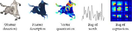
Fig. 5.1 Construction of bags of features for feature-based shape retrieval
5.1.1 Applications
Two archetypal problems in shape analysis addressed by feature-based methods are shape similarity and correspondence. The former underlies many pattern recognition applications, where we have to distinguish between different geometric objects (e.g. in 3D face recognition [15]). A particularly challenging setting of the shape similarity problem appears in content-based shape retrieval, an application driven by the availability of large public-domain databases of 3D models, such as Google 3D Warehouse, which have created the demand for shape search and retrieval algorithms capable of finding similar shapes in the same way a search engine responds to text queries (detailed discussion of this application appears in Chap. 7).
One of the notable advantages of feature-based approaches in shape retrieval is the possibility of representing a shape as a collection of primitive elements (“geometric words”), and using the well-developed methods from text search such as the bag of features (BOF) (or bag of words) paradigm [23, 75]. Such approaches are widely used in image retrieval and have been introduced more recently to shape analysis [19, 83]. The construction of a bag of features is usually performed in a few steps, depicted in Fig. 5.1. Firstly, the shape is represented as a collection of local feature descriptors (either dense or computed as a set of stable points following an optional stage of feature detection). Secondly, the descriptors are represented by geometric words from a geometric vocabulary using vector quantization. The geometric vocabulary is a set of representative descriptors, precomputed in advance. This way, each descriptor is replaced by the index of the closest geometric word in the vocabulary. Computing the histogram of the frequency of occurrence of geometric words gives the bag of features. Alternatively, a two-dimensional histogram of cooccurrences of pairs of geometric words (geometric expressions) can be used [19]. Shape similarity is computed as a distance between the corresponding bags of features. The bag of features representation is usually compact, easy to store and compare, which makes such approaches suitable for large-scale shape retrieval. Evaluation of shape retrieval performance (e.g. the robust large-scale retrieval benchmark [13] from the Shape Retrieval Contest (SHREC)) tests the robustness of retrieval algorithms on a large set of shapes with different simulated transformations, including non-rigid deformations.
Another fundamental problem in shape analysis is that of correspondence consisting of finding relations between similar points on two or more shapes. Finding
188 |
A.M. Bronstein et al. |
correspondence between two shapes that would be invariant to a wide variety of transformations is usually referred to as invariant shape correspondence. Correspondence problems are often encountered in shape synthesis applications such as morphing. In order to morph one shape into the other, one needs to know which point on the first shape will be transformed into a point on the second shape, in other words, establishing a correspondence between the shapes. A related problem is registration, where the deformation bringing one shape into the other is explicitly sought for.
Feature-based methods for shape correspondence are based on first detecting features on two shapes between which correspondence is sought, and then match them by comparing the corresponding descriptors. The feature-based correspondence problem can be formulated as finding a map that maximizes the similarity between corresponding descriptors. The caveat of such an approach is that it may produce inconsistent matches, especially in shapes with repeating structure or symmetry: for example, points on the right and left sides of a human body can be swapped due to bilateral symmetry. A way to cope with this problem is to add some global structure, for example, pairwise geodesic or diffusion distance preservation constraint. Thus, this type of minimum-distortion correspondence tries to match simultaneously local structures (descriptors) and global structures (metrics), and can be found by an extension of the generalized multidimensional scaling (GMDS) algorithm [16, 82] or graph labeling [78, 84, 85]. Evaluation of correspondence finding algorithms typically simulates a one-to-one shape matching scenario, in which one of the shapes undergoes multiple modifications and transformations, and the quality of the correspondence is evaluated as the distance on the shape between the found matches and the known groundtruth correspondence. Notable benchmarks are the SHREC robust correspondence benchmark [14] and the Princeton correspondence benchmark [41].
5.1.2 Chapter Outline
In this chapter, we present an overview of feature-based methods in 3D shape analysis and their applications, classical as well as most recent approaches. The main emphasis is on heat-kernel based detection and description algorithms, a relatively recent set of methods based on a common mathematical model and falling under the umbrella of diffusion geometry. Detailed description, examples, figures, and problems in this chapter allows the implementation of these methods.
The next section outlines some prerequisite mathematical background, describing our notation and a number of important concepts in differential and diffusion geometry. Then the two main sections are presented: Sect. 5.3 discusses feature detectors, while Sect. 5.4 describes feature descriptors. The final sections give concluding remarks, research challenges and suggested further reading.