f v1 v2 v3 v4 ...

Vertex/texture-coordinate. A vertex index may be followed by a texture coordinate index, separated by a slash.

f v1/vt1 v2/vt2 v3/vt3 ...

Vertex/texture-coordinate/normal. A vertex index may be followed by both a texture coordinate and surface normal index, each separated by a slash.

f v1/vt1/vn1 v2/vt2/vn2 v3/vt3/vn3 ...

Vertex/normal. A vertex index may be followed by only a surface normal index, separated by a double slash.

f v1//vn1 v2//vn2 v3//vn3 ...

An OBJ file may be augmented by a companion MTL (Material Template Library) file, which describes surface shading and material properties for the purposes of rendering.

4.3.2 Mesh Data Structures

To apply any processing to a mesh, such as rendering, manipulation or editing, we must be able to retrieve elements of the mesh and discover adjacency relationships. The most common such queries include: finding the faces/edges which are incident on a given vertex, finding the faces which border an edge, finding the edges which border a face, and finding the faces which are adjacent to a face. Mesh data structures can be classified according to how efficiently these queries can be answered. This is often traded off against storage overhead and representational power.

There are a large number of data structures available for the purpose of representing meshes. Some of the most common are summarized below.

Face list. A list of faces, each of which stores vertex positions. There is no redundancy in this representation, but connectivity between faces with shared vertices is not stored. Adjacency queries or transformations are inefficient and awkward.

Vertex-face list. A commonly used representation which is space efficient. It comprises a list of shared vertices and a list of faces, each of which stores pointers into the shared vertex list for each of its vertices. Since this is the representation used in most 3D file formats, such as OBJ, it is straightforward to load archival data into this structure.

Vertex-vertex list. A list of vertices, each containing a list to the vertices to which it is adjacent. Face and edge information is implicit and hence rendering is inefficient since it is necessary to traverse the structure to build lists of polygons. They are, however, extremely simple and are efficient when modeling complex changes in geometry [61].

Edge list. An edge list can be built from a vertex/face list in O(M) time for a mesh of M faces. An edge list is useful for a number of geometric computer graphics algorithms such as computing stencil shadows.

Table 4.2 Space and time complexity of mesh data structures for a mesh of M faces and N vertices

Winged-edge. The best known boundary representation (B-rep). Each edge stores pointers to the two vertices at their ends, the two faces bordering them, and pointers to four of the edges connected to the end points. This structure allows edge-vertex and edge-face queries to be answered in constant time, though other adjacency queries can require more processing.

Halfedge. Also known as the FE-structure [78] or as a doubly-connected edge list (DCEL) [4], although note that the originally proposed DCEL [43] described a different data structure. The halfedge is a B-rep structure which makes explicit the notion that an edge is shared by two faces by splitting an edge into two entities. It is restricted to representing manifold surfaces. Further implementation details are given below.

Adjacency matrix. A symmetric matrix of size N × N , which contains 1 if there is an edge between the corresponding vertices. Highly space inefficient for meshes but allows some operations to be performed by applying linear algebra to the adjacency matrix. This forms the basis of algebraic graph theory [5].

We provide a summary of the time and space complexity of a representative sample of mesh data structures in Table 4.2. Note that different structures that support operations with the same asymptotic complexity, may not be equally efficient in practice. For example, finding all vertices of a face using a winged-edge structure requires traversal from the face list to the edge list to the vertex list, whereas the vertex-face list structure can traverse directly from faces to vertices. Also note that, where we specify constant time, we refer to constant time per piece of information. So, for example, using a halfedge all of the edges incident on a vertex can be computed in a time which is linear in the number of edges incident on the vertex.

The halfedge structure allows all adjacency queries to be computed in constant time, while requiring only a modest overhead in storage requirements. For this reason, it is a good choice as a general purpose data structure for mesh processing. We describe the halfedge data structure in more detail in the following sections.

4.3.2.1 Halfedge Structure

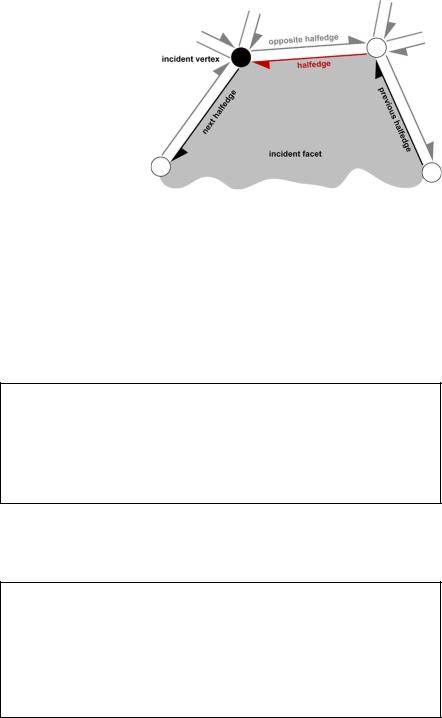
The halfedge data structure comprises vertices, faces and “halfedges”. Each edge in the mesh is represented by two halfedges. Conceptually, a halfedge is obtained by dividing an edge down its length. Figure 4.11 shows a small section of a mesh represented using the halfedge structure. Halfedges store pointers to the following:

Fig. 4.11 Halfedge structure

1.The next halfedge in the facet (and so they form a circularly linked list around the face).

2.Its companion “opposite” halfedge.

3.The vertex at the end of the halfedge.

4.The face that the halfedge borders.

Note that halfedges can be linked in clockwise or counterclockwise direction about a face, but this must be consistent over the mesh.

Concretely, in the C programming language, a minimal halfedge structure would be implemented as follows:

s t r u c t h a l f e d g e

{

h a l f e d g e n e x t ;

h a l f e d g e o p p o s i t e ;

v e r t e x i n c i d e n t v e r t e x ; f a c e i n c i d e n t f a c e t ;

} ;

In the halfedge data structure, a vertex stores 3D position (as well as any other pervertex information) and a pointer to one of the halfedges that uses the vertex as a starting point:

s t r u c t v e r t e x

/ / A d d i t i o n a l per−v e r t e x d a t a h e r e h a l f e d g e o u t g o i n g e d g e ;

}

Finally, a facet stores any per-facet information (for example, face normals) and a pointer to one of the halfedges bordering the face:

s t r u c t f a c e

{

/ / A d d i t i o n a l per− f a c e t d a t a h e r e h a l f e d g e b o r d e r e d g e ;

}

With the halfedge structure to hand, traversals are achieved by simply following the appropriate pointers. In the simplest case, the vertices adjacent to an edge can be found as follows:

A similar approach can be applied for adjacent faces. Traversing the perimeter of a face is simply a case of following a circularly linked list:

h a l f e d g e e d g e = f a c e −>b o r d e r e d g e ;

Another useful operation is iterating over all the edges adjacent to a vertex (this is important for range searching and also for vertex deletion resulting from an edge collapse, where pointers to this vertex must be changed to point to the vertex at the other end of the deleted edge). This is implemented as follows:

h a l f e d g e e d g e = v e r t −>o u t g o i n g e d g e ;

Many other traversal operations can be implemented in a similar manner. In the context of range searching, edge lengths need to be considered (i.e. the Euclidean distance between adjacent vertices). Dijkstra’s shortest path algorithm can be applied in this context for range searching using approximate geodesic distances or for exact geodesic distances the Fast Marching Method can be used [30]. Exercise 7 asks you to implement Dijkstra’s shortest path algorithm on a halfedge structure.