

- •Preface
- •Biological Vision Systems
- •Visual Representations from Paintings to Photographs
- •Computer Vision
- •The Limitations of Standard 2D Images
- •3D Imaging, Analysis and Applications
- •Book Objective and Content
- •Acknowledgements
- •Contents
- •Contributors
- •2.1 Introduction
- •Chapter Outline
- •2.2 An Overview of Passive 3D Imaging Systems
- •2.2.1 Multiple View Approaches
- •2.2.2 Single View Approaches
- •2.3 Camera Modeling
- •2.3.1 Homogeneous Coordinates
- •2.3.2 Perspective Projection Camera Model
- •2.3.2.1 Camera Modeling: The Coordinate Transformation
- •2.3.2.2 Camera Modeling: Perspective Projection
- •2.3.2.3 Camera Modeling: Image Sampling
- •2.3.2.4 Camera Modeling: Concatenating the Projective Mappings
- •2.3.3 Radial Distortion
- •2.4 Camera Calibration
- •2.4.1 Estimation of a Scene-to-Image Planar Homography
- •2.4.2 Basic Calibration
- •2.4.3 Refined Calibration
- •2.4.4 Calibration of a Stereo Rig
- •2.5 Two-View Geometry
- •2.5.1 Epipolar Geometry
- •2.5.2 Essential and Fundamental Matrices
- •2.5.3 The Fundamental Matrix for Pure Translation
- •2.5.4 Computation of the Fundamental Matrix
- •2.5.5 Two Views Separated by a Pure Rotation
- •2.5.6 Two Views of a Planar Scene
- •2.6 Rectification
- •2.6.1 Rectification with Calibration Information
- •2.6.2 Rectification Without Calibration Information
- •2.7 Finding Correspondences
- •2.7.1 Correlation-Based Methods
- •2.7.2 Feature-Based Methods
- •2.8 3D Reconstruction
- •2.8.1 Stereo
- •2.8.1.1 Dense Stereo Matching
- •2.8.1.2 Triangulation
- •2.8.2 Structure from Motion
- •2.9 Passive Multiple-View 3D Imaging Systems
- •2.9.1 Stereo Cameras
- •2.9.2 3D Modeling
- •2.9.3 Mobile Robot Localization and Mapping
- •2.10 Passive Versus Active 3D Imaging Systems
- •2.11 Concluding Remarks
- •2.12 Further Reading
- •2.13 Questions
- •2.14 Exercises
- •References
- •3.1 Introduction
- •3.1.1 Historical Context
- •3.1.2 Basic Measurement Principles
- •3.1.3 Active Triangulation-Based Methods
- •3.1.4 Chapter Outline
- •3.2 Spot Scanners
- •3.2.1 Spot Position Detection
- •3.3 Stripe Scanners
- •3.3.1 Camera Model
- •3.3.2 Sheet-of-Light Projector Model
- •3.3.3 Triangulation for Stripe Scanners
- •3.4 Area-Based Structured Light Systems
- •3.4.1 Gray Code Methods
- •3.4.1.1 Decoding of Binary Fringe-Based Codes
- •3.4.1.2 Advantage of the Gray Code
- •3.4.2 Phase Shift Methods
- •3.4.2.1 Removing the Phase Ambiguity
- •3.4.3 Triangulation for a Structured Light System
- •3.5 System Calibration
- •3.6 Measurement Uncertainty
- •3.6.1 Uncertainty Related to the Phase Shift Algorithm
- •3.6.2 Uncertainty Related to Intrinsic Parameters
- •3.6.3 Uncertainty Related to Extrinsic Parameters
- •3.6.4 Uncertainty as a Design Tool
- •3.7 Experimental Characterization of 3D Imaging Systems
- •3.7.1 Low-Level Characterization
- •3.7.2 System-Level Characterization
- •3.7.3 Characterization of Errors Caused by Surface Properties
- •3.7.4 Application-Based Characterization
- •3.8 Selected Advanced Topics
- •3.8.1 Thin Lens Equation
- •3.8.2 Depth of Field
- •3.8.3 Scheimpflug Condition
- •3.8.4 Speckle and Uncertainty
- •3.8.5 Laser Depth of Field
- •3.8.6 Lateral Resolution
- •3.9 Research Challenges
- •3.10 Concluding Remarks
- •3.11 Further Reading
- •3.12 Questions
- •3.13 Exercises
- •References
- •4.1 Introduction
- •Chapter Outline
- •4.2 Representation of 3D Data
- •4.2.1 Raw Data
- •4.2.1.1 Point Cloud
- •4.2.1.2 Structured Point Cloud
- •4.2.1.3 Depth Maps and Range Images
- •4.2.1.4 Needle map
- •4.2.1.5 Polygon Soup
- •4.2.2 Surface Representations
- •4.2.2.1 Triangular Mesh
- •4.2.2.2 Quadrilateral Mesh
- •4.2.2.3 Subdivision Surfaces
- •4.2.2.4 Morphable Model
- •4.2.2.5 Implicit Surface
- •4.2.2.6 Parametric Surface
- •4.2.2.7 Comparison of Surface Representations
- •4.2.3 Solid-Based Representations
- •4.2.3.1 Voxels
- •4.2.3.3 Binary Space Partitioning
- •4.2.3.4 Constructive Solid Geometry
- •4.2.3.5 Boundary Representations
- •4.2.4 Summary of Solid-Based Representations
- •4.3 Polygon Meshes
- •4.3.1 Mesh Storage
- •4.3.2 Mesh Data Structures
- •4.3.2.1 Halfedge Structure
- •4.4 Subdivision Surfaces
- •4.4.1 Doo-Sabin Scheme
- •4.4.2 Catmull-Clark Scheme
- •4.4.3 Loop Scheme
- •4.5 Local Differential Properties
- •4.5.1 Surface Normals
- •4.5.2 Differential Coordinates and the Mesh Laplacian
- •4.6 Compression and Levels of Detail
- •4.6.1 Mesh Simplification
- •4.6.1.1 Edge Collapse
- •4.6.1.2 Quadric Error Metric
- •4.6.2 QEM Simplification Summary
- •4.6.3 Surface Simplification Results
- •4.7 Visualization
- •4.8 Research Challenges
- •4.9 Concluding Remarks
- •4.10 Further Reading
- •4.11 Questions
- •4.12 Exercises
- •References
- •1.1 Introduction
- •Chapter Outline
- •1.2 A Historical Perspective on 3D Imaging
- •1.2.1 Image Formation and Image Capture
- •1.2.2 Binocular Perception of Depth
- •1.2.3 Stereoscopic Displays
- •1.3 The Development of Computer Vision
- •1.3.1 Further Reading in Computer Vision
- •1.4 Acquisition Techniques for 3D Imaging
- •1.4.1 Passive 3D Imaging
- •1.4.2 Active 3D Imaging
- •1.4.3 Passive Stereo Versus Active Stereo Imaging
- •1.5 Twelve Milestones in 3D Imaging and Shape Analysis
- •1.5.1 Active 3D Imaging: An Early Optical Triangulation System
- •1.5.2 Passive 3D Imaging: An Early Stereo System
- •1.5.3 Passive 3D Imaging: The Essential Matrix
- •1.5.4 Model Fitting: The RANSAC Approach to Feature Correspondence Analysis
- •1.5.5 Active 3D Imaging: Advances in Scanning Geometries
- •1.5.6 3D Registration: Rigid Transformation Estimation from 3D Correspondences
- •1.5.7 3D Registration: Iterative Closest Points
- •1.5.9 3D Local Shape Descriptors: Spin Images
- •1.5.10 Passive 3D Imaging: Flexible Camera Calibration
- •1.5.11 3D Shape Matching: Heat Kernel Signatures
- •1.6 Applications of 3D Imaging
- •1.7 Book Outline
- •1.7.1 Part I: 3D Imaging and Shape Representation
- •1.7.2 Part II: 3D Shape Analysis and Processing
- •1.7.3 Part III: 3D Imaging Applications
- •References
- •5.1 Introduction
- •5.1.1 Applications
- •5.1.2 Chapter Outline
- •5.2 Mathematical Background
- •5.2.1 Differential Geometry
- •5.2.2 Curvature of Two-Dimensional Surfaces
- •5.2.3 Discrete Differential Geometry
- •5.2.4 Diffusion Geometry
- •5.2.5 Discrete Diffusion Geometry
- •5.3 Feature Detectors
- •5.3.1 A Taxonomy
- •5.3.2 Harris 3D
- •5.3.3 Mesh DOG
- •5.3.4 Salient Features
- •5.3.5 Heat Kernel Features
- •5.3.6 Topological Features
- •5.3.7 Maximally Stable Components
- •5.3.8 Benchmarks
- •5.4 Feature Descriptors
- •5.4.1 A Taxonomy
- •5.4.2 Curvature-Based Descriptors (HK and SC)
- •5.4.3 Spin Images
- •5.4.4 Shape Context
- •5.4.5 Integral Volume Descriptor
- •5.4.6 Mesh Histogram of Gradients (HOG)
- •5.4.7 Heat Kernel Signature (HKS)
- •5.4.8 Scale-Invariant Heat Kernel Signature (SI-HKS)
- •5.4.9 Color Heat Kernel Signature (CHKS)
- •5.4.10 Volumetric Heat Kernel Signature (VHKS)
- •5.5 Research Challenges
- •5.6 Conclusions
- •5.7 Further Reading
- •5.8 Questions
- •5.9 Exercises
- •References
- •6.1 Introduction
- •Chapter Outline
- •6.2 Registration of Two Views
- •6.2.1 Problem Statement
- •6.2.2 The Iterative Closest Points (ICP) Algorithm
- •6.2.3 ICP Extensions
- •6.2.3.1 Techniques for Pre-alignment
- •Global Approaches
- •Local Approaches
- •6.2.3.2 Techniques for Improving Speed
- •Subsampling
- •Closest Point Computation
- •Distance Formulation
- •6.2.3.3 Techniques for Improving Accuracy
- •Outlier Rejection
- •Additional Information
- •Probabilistic Methods
- •6.3 Advanced Techniques
- •6.3.1 Registration of More than Two Views
- •Reducing Error Accumulation
- •Automating Registration
- •6.3.2 Registration in Cluttered Scenes
- •Point Signatures
- •Matching Methods
- •6.3.3 Deformable Registration
- •Methods Based on General Optimization Techniques
- •Probabilistic Methods
- •6.3.4 Machine Learning Techniques
- •Improving the Matching
- •Object Detection
- •6.4 Quantitative Performance Evaluation
- •6.5 Case Study 1: Pairwise Alignment with Outlier Rejection
- •6.6 Case Study 2: ICP with Levenberg-Marquardt
- •6.6.1 The LM-ICP Method
- •6.6.2 Computing the Derivatives
- •6.6.3 The Case of Quaternions
- •6.6.4 Summary of the LM-ICP Algorithm
- •6.6.5 Results and Discussion
- •6.7 Case Study 3: Deformable ICP with Levenberg-Marquardt
- •6.7.1 Surface Representation
- •6.7.2 Cost Function
- •Data Term: Global Surface Attraction
- •Data Term: Boundary Attraction
- •Penalty Term: Spatial Smoothness
- •Penalty Term: Temporal Smoothness
- •6.7.3 Minimization Procedure
- •6.7.4 Summary of the Algorithm
- •6.7.5 Experiments
- •6.8 Research Challenges
- •6.9 Concluding Remarks
- •6.10 Further Reading
- •6.11 Questions
- •6.12 Exercises
- •References
- •7.1 Introduction
- •7.1.1 Retrieval and Recognition Evaluation
- •7.1.2 Chapter Outline
- •7.2 Literature Review
- •7.3 3D Shape Retrieval Techniques
- •7.3.1 Depth-Buffer Descriptor
- •7.3.1.1 Computing the 2D Projections
- •7.3.1.2 Obtaining the Feature Vector
- •7.3.1.3 Evaluation
- •7.3.1.4 Complexity Analysis
- •7.3.2 Spin Images for Object Recognition
- •7.3.2.1 Matching
- •7.3.2.2 Evaluation
- •7.3.2.3 Complexity Analysis
- •7.3.3 Salient Spectral Geometric Features
- •7.3.3.1 Feature Points Detection
- •7.3.3.2 Local Descriptors
- •7.3.3.3 Shape Matching
- •7.3.3.4 Evaluation
- •7.3.3.5 Complexity Analysis
- •7.3.4 Heat Kernel Signatures
- •7.3.4.1 Evaluation
- •7.3.4.2 Complexity Analysis
- •7.4 Research Challenges
- •7.5 Concluding Remarks
- •7.6 Further Reading
- •7.7 Questions
- •7.8 Exercises
- •References
- •8.1 Introduction
- •Chapter Outline
- •8.2 3D Face Scan Representation and Visualization
- •8.3 3D Face Datasets
- •8.3.1 FRGC v2 3D Face Dataset
- •8.3.2 The Bosphorus Dataset
- •8.4 3D Face Recognition Evaluation
- •8.4.1 Face Verification
- •8.4.2 Face Identification
- •8.5 Processing Stages in 3D Face Recognition
- •8.5.1 Face Detection and Segmentation
- •8.5.2 Removal of Spikes
- •8.5.3 Filling of Holes and Missing Data
- •8.5.4 Removal of Noise
- •8.5.5 Fiducial Point Localization and Pose Correction
- •8.5.6 Spatial Resampling
- •8.5.7 Feature Extraction on Facial Surfaces
- •8.5.8 Classifiers for 3D Face Matching
- •8.6 ICP-Based 3D Face Recognition
- •8.6.1 ICP Outline
- •8.6.2 A Critical Discussion of ICP
- •8.6.3 A Typical ICP-Based 3D Face Recognition Implementation
- •8.6.4 ICP Variants and Other Surface Registration Approaches
- •8.7 PCA-Based 3D Face Recognition
- •8.7.1 PCA System Training
- •8.7.2 PCA Training Using Singular Value Decomposition
- •8.7.3 PCA Testing
- •8.7.4 PCA Performance
- •8.8 LDA-Based 3D Face Recognition
- •8.8.1 Two-Class LDA
- •8.8.2 LDA with More than Two Classes
- •8.8.3 LDA in High Dimensional 3D Face Spaces
- •8.8.4 LDA Performance
- •8.9 Normals and Curvature in 3D Face Recognition
- •8.9.1 Computing Curvature on a 3D Face Scan
- •8.10 Recent Techniques in 3D Face Recognition
- •8.10.1 3D Face Recognition Using Annotated Face Models (AFM)
- •8.10.2 Local Feature-Based 3D Face Recognition
- •8.10.2.1 Keypoint Detection and Local Feature Matching
- •8.10.2.2 Other Local Feature-Based Methods
- •8.10.3 Expression Modeling for Invariant 3D Face Recognition
- •8.10.3.1 Other Expression Modeling Approaches
- •8.11 Research Challenges
- •8.12 Concluding Remarks
- •8.13 Further Reading
- •8.14 Questions
- •8.15 Exercises
- •References
- •9.1 Introduction
- •Chapter Outline
- •9.2 DEM Generation from Stereoscopic Imagery
- •9.2.1 Stereoscopic DEM Generation: Literature Review
- •9.2.2 Accuracy Evaluation of DEMs
- •9.2.3 An Example of DEM Generation from SPOT-5 Imagery
- •9.3 DEM Generation from InSAR
- •9.3.1 Techniques for DEM Generation from InSAR
- •9.3.1.1 Basic Principle of InSAR in Elevation Measurement
- •9.3.1.2 Processing Stages of DEM Generation from InSAR
- •The Branch-Cut Method of Phase Unwrapping
- •The Least Squares (LS) Method of Phase Unwrapping
- •9.3.2 Accuracy Analysis of DEMs Generated from InSAR
- •9.3.3 Examples of DEM Generation from InSAR
- •9.4 DEM Generation from LIDAR
- •9.4.1 LIDAR Data Acquisition
- •9.4.2 Accuracy, Error Types and Countermeasures
- •9.4.3 LIDAR Interpolation
- •9.4.4 LIDAR Filtering
- •9.4.5 DTM from Statistical Properties of the Point Cloud
- •9.5 Research Challenges
- •9.6 Concluding Remarks
- •9.7 Further Reading
- •9.8 Questions
- •9.9 Exercises
- •References
- •10.1 Introduction
- •10.1.1 Allometric Modeling of Biomass
- •10.1.2 Chapter Outline
- •10.2 Aerial Photo Mensuration
- •10.2.1 Principles of Aerial Photogrammetry
- •10.2.1.1 Geometric Basis of Photogrammetric Measurement
- •10.2.1.2 Ground Control and Direct Georeferencing
- •10.2.2 Tree Height Measurement Using Forest Photogrammetry
- •10.2.2.2 Automated Methods in Forest Photogrammetry
- •10.3 Airborne Laser Scanning
- •10.3.1 Principles of Airborne Laser Scanning
- •10.3.1.1 Lidar-Based Measurement of Terrain and Canopy Surfaces
- •10.3.2 Individual Tree-Level Measurement Using Lidar
- •10.3.2.1 Automated Individual Tree Measurement Using Lidar
- •10.3.3 Area-Based Approach to Estimating Biomass with Lidar
- •10.4 Future Developments
- •10.5 Concluding Remarks
- •10.6 Further Reading
- •10.7 Questions
- •References
- •11.1 Introduction
- •Chapter Outline
- •11.2 Volumetric Data Acquisition
- •11.2.1 Computed Tomography
- •11.2.1.1 Characteristics of 3D CT Data
- •11.2.2 Positron Emission Tomography (PET)
- •11.2.2.1 Characteristics of 3D PET Data
- •Relaxation
- •11.2.3.1 Characteristics of the 3D MRI Data
- •Image Quality and Artifacts
- •11.2.4 Summary
- •11.3 Surface Extraction and Volumetric Visualization
- •11.3.1 Surface Extraction
- •Example: Curvatures and Geometric Tools
- •11.3.2 Volume Rendering
- •11.3.3 Summary
- •11.4 Volumetric Image Registration
- •11.4.1 A Hierarchy of Transformations
- •11.4.1.1 Rigid Body Transformation
- •11.4.1.2 Similarity Transformations and Anisotropic Scaling
- •11.4.1.3 Affine Transformations
- •11.4.1.4 Perspective Transformations
- •11.4.1.5 Non-rigid Transformations
- •11.4.2 Points and Features Used for the Registration
- •11.4.2.1 Landmark Features
- •11.4.2.2 Surface-Based Registration
- •11.4.2.3 Intensity-Based Registration
- •11.4.3 Registration Optimization
- •11.4.3.1 Estimation of Registration Errors
- •11.4.4 Summary
- •11.5 Segmentation
- •11.5.1 Semi-automatic Methods
- •11.5.1.1 Thresholding
- •11.5.1.2 Region Growing
- •11.5.1.3 Deformable Models
- •Snakes
- •Balloons
- •11.5.2 Fully Automatic Methods
- •11.5.2.1 Atlas-Based Segmentation
- •11.5.2.2 Statistical Shape Modeling and Analysis
- •11.5.3 Summary
- •11.6 Diffusion Imaging: An Illustration of a Full Pipeline
- •11.6.1 From Scalar Images to Tensors
- •11.6.2 From Tensor Image to Information
- •11.6.3 Summary
- •11.7 Applications
- •11.7.1 Diagnosis and Morphometry
- •11.7.2 Simulation and Training
- •11.7.3 Surgical Planning and Guidance
- •11.7.4 Summary
- •11.8 Concluding Remarks
- •11.9 Research Challenges
- •11.10 Further Reading
- •Data Acquisition
- •Surface Extraction
- •Volume Registration
- •Segmentation
- •Diffusion Imaging
- •Software
- •11.11 Questions
- •11.12 Exercises
- •References
- •Index

468 |
P.G. Batchelor et al. |
tive measurements of blood flow or electrical activation [72]; in image-guided interventions, segmentations are often required for visualization in surgical planning or guidance [63]. Segmentation techniques have been applied to delineate a wide variety of organs from medical imaging data acquired using a wide range of modalities.
Approaches to segmentation vary a lot in terms of their sophistication and the amount of user input required. Purely manual techniques allow users to outline structures using software such as the ANALYZE1 package. Manual segmentation can be very accurate, but time-consuming, and is subject to inter-observer variation or bias. Semi-automatic techniques allow the user to have some control or input into the segmentation process, combined with automatic processing using computer algorithms. Finally, fully automatic techniques require no user input and often make use of some prior knowledge to produce the segmentation. The following sections review a number of semi-automatic and fully automatic approaches to medical image segmentation. Our coverage of this huge research area is not exhaustive, but we provide a few examples that give an introduction to the field.
11.5.1 Semi-automatic Methods
In this section, we consider three semi-automatic approaches to segmentation based on thresholding, region growing and deformable models.
11.5.1.1 Thresholding
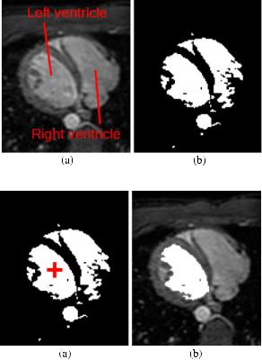
Perhaps the simplest example of user interaction in segmentation is the specification of a threshold. Typically, a thresholding operation involves comparing every intensity in the image to the threshold value and setting it to 1 if it is greater than or equal to the threshold, or 0 otherwise, thereby creating a binary image. Figure 11.13 illustrates this operation on cardiac MRI data. Software such as ITKSNAP can be used to interactively adjust the threshold to produce the desired result. Thresholding is commonly applied as one step in a segmentation pipeline, but the presence of noise, image artifacts and other structures in the image mean that it is rarely enough on its own to produce an accurate and reliable segmentation. This fact can be observed in Fig. 11.13b, in which several pixels outside of the left and right ventricles are set to 1, despite not being the target structures of the segmentation.
1Biomedical Imaging Resource, Mayo Foundation, Rochester, MN, USA or ITK-SNAP [84], http://www.itksnap.org.
11 3D Medical Imaging |
469 |
Fig. 11.13 Thresholding an axial cardiac MRI slice.
(a) Original slice. (b) Result of thresholding operation
Fig. 11.14 Segmenting the left ventricle using region growing on the thresholded axial cardiac MR slice.
(a) Thresholded image with seed point in the left ventricle indicated by the red cross. (b) Result of region growing, overlaid onto original cardiac MRI slice
11.5.1.2 Region Growing
One technique that can be used to refine thresholded images, such as that shown in Fig. 11.13b, is known as region growing. Region growing involves user interaction in the form of specifying a seed point. This is a pixel in the image that is known to lie inside the structure being segmented. The region is then iteratively grown by adding neighboring pixels that have similar appearance. The concept of similarity needs to be defined: for example, by specifying a range of intensity values around that of the seed pixel. If region growing is applied to a thresholded image then, to be considered similar, pixels should have the same binary value as the seed pixels. In addition, the concept of neighborhood needs to be defined, with 4-neighborhoods (i.e. only directly adjacent pixels) and 8-neighborhoods (i.e. including diagonally adjacent) commonly used in 2D images. Figure 11.14 illustrates the operation of the region growing algorithm for segmenting the left ventricle from the cardiac MRI data introduced in Fig. 11.13. A seed point has been placed in the left ventricle (indicated by the red cross) and the region growing algorithm has included all pixels that were connected to this seed, excluding all others. The resulting segmentation is of the left ventricle only.
470 |
P.G. Batchelor et al. |
Algorithm 11.1 REGION GROW on seed pixel Require: Initialize all pixels to unknown region
Set current pixel to be inside region for all neighboring pixels do
if it is inside image bounds and currently has an unknown region then Compute similarity to current pixel
if similar then
REGION GROW on neighboring pixel else
Set neighboring pixel to background end if
end if end for
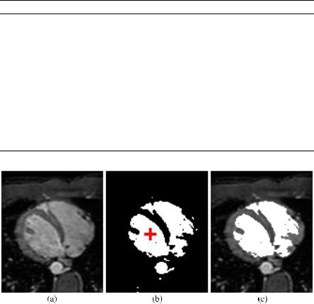
Fig. 11.15 The problem of leaks in region growing. (a) An axial cardiac MRI slice. (b) Result of thresholding operation, seed point for region growing in the left ventricle indicated by the red cross. (c) Result of region growing. The segmentation has ‘leaked’ into the right ventricle
The region growing algorithm can be implemented in a number of ways. The simplest, although not the most computationally efficient, is a recursive implementation. There are many implementations and this is the same problem as flood-fill or area-fill in graphics or vision. Pseudocode for recursive region growing is given in Algorithm 11.1.
One problem that the region growing algorithm can encounter is that of leaks. This problem is illustrated in Fig. 11.15. This shows a different axial cardiac MRI slice from that used in Fig. 11.13 and Fig. 11.14. This time the region growing has ‘leaked’ the segmentation into the right ventricle. Therefore, in region growing, care must be taken when selecting threshold values and specifying the similarity term to avoid such cases. The region growing algorithm can be extended to 3D, in which case the neighborhood in Algorithm 11.1 will extend to 3D accordingly. However, in 3D the problem of leaks can be exacerbated.