
- •Preface
- •Biological Vision Systems
- •Visual Representations from Paintings to Photographs
- •Computer Vision
- •The Limitations of Standard 2D Images
- •3D Imaging, Analysis and Applications
- •Book Objective and Content
- •Acknowledgements
- •Contents
- •Contributors
- •2.1 Introduction
- •Chapter Outline
- •2.2 An Overview of Passive 3D Imaging Systems
- •2.2.1 Multiple View Approaches
- •2.2.2 Single View Approaches
- •2.3 Camera Modeling
- •2.3.1 Homogeneous Coordinates
- •2.3.2 Perspective Projection Camera Model
- •2.3.2.1 Camera Modeling: The Coordinate Transformation
- •2.3.2.2 Camera Modeling: Perspective Projection
- •2.3.2.3 Camera Modeling: Image Sampling
- •2.3.2.4 Camera Modeling: Concatenating the Projective Mappings
- •2.3.3 Radial Distortion
- •2.4 Camera Calibration
- •2.4.1 Estimation of a Scene-to-Image Planar Homography
- •2.4.2 Basic Calibration
- •2.4.3 Refined Calibration
- •2.4.4 Calibration of a Stereo Rig
- •2.5 Two-View Geometry
- •2.5.1 Epipolar Geometry
- •2.5.2 Essential and Fundamental Matrices
- •2.5.3 The Fundamental Matrix for Pure Translation
- •2.5.4 Computation of the Fundamental Matrix
- •2.5.5 Two Views Separated by a Pure Rotation
- •2.5.6 Two Views of a Planar Scene
- •2.6 Rectification
- •2.6.1 Rectification with Calibration Information
- •2.6.2 Rectification Without Calibration Information
- •2.7 Finding Correspondences
- •2.7.1 Correlation-Based Methods
- •2.7.2 Feature-Based Methods
- •2.8 3D Reconstruction
- •2.8.1 Stereo
- •2.8.1.1 Dense Stereo Matching
- •2.8.1.2 Triangulation
- •2.8.2 Structure from Motion
- •2.9 Passive Multiple-View 3D Imaging Systems
- •2.9.1 Stereo Cameras
- •2.9.2 3D Modeling
- •2.9.3 Mobile Robot Localization and Mapping
- •2.10 Passive Versus Active 3D Imaging Systems
- •2.11 Concluding Remarks
- •2.12 Further Reading
- •2.13 Questions
- •2.14 Exercises
- •References
- •3.1 Introduction
- •3.1.1 Historical Context
- •3.1.2 Basic Measurement Principles
- •3.1.3 Active Triangulation-Based Methods
- •3.1.4 Chapter Outline
- •3.2 Spot Scanners
- •3.2.1 Spot Position Detection
- •3.3 Stripe Scanners
- •3.3.1 Camera Model
- •3.3.2 Sheet-of-Light Projector Model
- •3.3.3 Triangulation for Stripe Scanners
- •3.4 Area-Based Structured Light Systems
- •3.4.1 Gray Code Methods
- •3.4.1.1 Decoding of Binary Fringe-Based Codes
- •3.4.1.2 Advantage of the Gray Code
- •3.4.2 Phase Shift Methods
- •3.4.2.1 Removing the Phase Ambiguity
- •3.4.3 Triangulation for a Structured Light System
- •3.5 System Calibration
- •3.6 Measurement Uncertainty
- •3.6.1 Uncertainty Related to the Phase Shift Algorithm
- •3.6.2 Uncertainty Related to Intrinsic Parameters
- •3.6.3 Uncertainty Related to Extrinsic Parameters
- •3.6.4 Uncertainty as a Design Tool
- •3.7 Experimental Characterization of 3D Imaging Systems
- •3.7.1 Low-Level Characterization
- •3.7.2 System-Level Characterization
- •3.7.3 Characterization of Errors Caused by Surface Properties
- •3.7.4 Application-Based Characterization
- •3.8 Selected Advanced Topics
- •3.8.1 Thin Lens Equation
- •3.8.2 Depth of Field
- •3.8.3 Scheimpflug Condition
- •3.8.4 Speckle and Uncertainty
- •3.8.5 Laser Depth of Field
- •3.8.6 Lateral Resolution
- •3.9 Research Challenges
- •3.10 Concluding Remarks
- •3.11 Further Reading
- •3.12 Questions
- •3.13 Exercises
- •References
- •4.1 Introduction
- •Chapter Outline
- •4.2 Representation of 3D Data
- •4.2.1 Raw Data
- •4.2.1.1 Point Cloud
- •4.2.1.2 Structured Point Cloud
- •4.2.1.3 Depth Maps and Range Images
- •4.2.1.4 Needle map
- •4.2.1.5 Polygon Soup
- •4.2.2 Surface Representations
- •4.2.2.1 Triangular Mesh
- •4.2.2.2 Quadrilateral Mesh
- •4.2.2.3 Subdivision Surfaces
- •4.2.2.4 Morphable Model
- •4.2.2.5 Implicit Surface
- •4.2.2.6 Parametric Surface
- •4.2.2.7 Comparison of Surface Representations
- •4.2.3 Solid-Based Representations
- •4.2.3.1 Voxels
- •4.2.3.3 Binary Space Partitioning
- •4.2.3.4 Constructive Solid Geometry
- •4.2.3.5 Boundary Representations
- •4.2.4 Summary of Solid-Based Representations
- •4.3 Polygon Meshes
- •4.3.1 Mesh Storage
- •4.3.2 Mesh Data Structures
- •4.3.2.1 Halfedge Structure
- •4.4 Subdivision Surfaces
- •4.4.1 Doo-Sabin Scheme
- •4.4.2 Catmull-Clark Scheme
- •4.4.3 Loop Scheme
- •4.5 Local Differential Properties
- •4.5.1 Surface Normals
- •4.5.2 Differential Coordinates and the Mesh Laplacian
- •4.6 Compression and Levels of Detail
- •4.6.1 Mesh Simplification
- •4.6.1.1 Edge Collapse
- •4.6.1.2 Quadric Error Metric
- •4.6.2 QEM Simplification Summary
- •4.6.3 Surface Simplification Results
- •4.7 Visualization
- •4.8 Research Challenges
- •4.9 Concluding Remarks
- •4.10 Further Reading
- •4.11 Questions
- •4.12 Exercises
- •References
- •1.1 Introduction
- •Chapter Outline
- •1.2 A Historical Perspective on 3D Imaging
- •1.2.1 Image Formation and Image Capture
- •1.2.2 Binocular Perception of Depth
- •1.2.3 Stereoscopic Displays
- •1.3 The Development of Computer Vision
- •1.3.1 Further Reading in Computer Vision
- •1.4 Acquisition Techniques for 3D Imaging
- •1.4.1 Passive 3D Imaging
- •1.4.2 Active 3D Imaging
- •1.4.3 Passive Stereo Versus Active Stereo Imaging
- •1.5 Twelve Milestones in 3D Imaging and Shape Analysis
- •1.5.1 Active 3D Imaging: An Early Optical Triangulation System
- •1.5.2 Passive 3D Imaging: An Early Stereo System
- •1.5.3 Passive 3D Imaging: The Essential Matrix
- •1.5.4 Model Fitting: The RANSAC Approach to Feature Correspondence Analysis
- •1.5.5 Active 3D Imaging: Advances in Scanning Geometries
- •1.5.6 3D Registration: Rigid Transformation Estimation from 3D Correspondences
- •1.5.7 3D Registration: Iterative Closest Points
- •1.5.9 3D Local Shape Descriptors: Spin Images
- •1.5.10 Passive 3D Imaging: Flexible Camera Calibration
- •1.5.11 3D Shape Matching: Heat Kernel Signatures
- •1.6 Applications of 3D Imaging
- •1.7 Book Outline
- •1.7.1 Part I: 3D Imaging and Shape Representation
- •1.7.2 Part II: 3D Shape Analysis and Processing
- •1.7.3 Part III: 3D Imaging Applications
- •References
- •5.1 Introduction
- •5.1.1 Applications
- •5.1.2 Chapter Outline
- •5.2 Mathematical Background
- •5.2.1 Differential Geometry
- •5.2.2 Curvature of Two-Dimensional Surfaces
- •5.2.3 Discrete Differential Geometry
- •5.2.4 Diffusion Geometry
- •5.2.5 Discrete Diffusion Geometry
- •5.3 Feature Detectors
- •5.3.1 A Taxonomy
- •5.3.2 Harris 3D
- •5.3.3 Mesh DOG
- •5.3.4 Salient Features
- •5.3.5 Heat Kernel Features
- •5.3.6 Topological Features
- •5.3.7 Maximally Stable Components
- •5.3.8 Benchmarks
- •5.4 Feature Descriptors
- •5.4.1 A Taxonomy
- •5.4.2 Curvature-Based Descriptors (HK and SC)
- •5.4.3 Spin Images
- •5.4.4 Shape Context
- •5.4.5 Integral Volume Descriptor
- •5.4.6 Mesh Histogram of Gradients (HOG)
- •5.4.7 Heat Kernel Signature (HKS)
- •5.4.8 Scale-Invariant Heat Kernel Signature (SI-HKS)
- •5.4.9 Color Heat Kernel Signature (CHKS)
- •5.4.10 Volumetric Heat Kernel Signature (VHKS)
- •5.5 Research Challenges
- •5.6 Conclusions
- •5.7 Further Reading
- •5.8 Questions
- •5.9 Exercises
- •References
- •6.1 Introduction
- •Chapter Outline
- •6.2 Registration of Two Views
- •6.2.1 Problem Statement
- •6.2.2 The Iterative Closest Points (ICP) Algorithm
- •6.2.3 ICP Extensions
- •6.2.3.1 Techniques for Pre-alignment
- •Global Approaches
- •Local Approaches
- •6.2.3.2 Techniques for Improving Speed
- •Subsampling
- •Closest Point Computation
- •Distance Formulation
- •6.2.3.3 Techniques for Improving Accuracy
- •Outlier Rejection
- •Additional Information
- •Probabilistic Methods
- •6.3 Advanced Techniques
- •6.3.1 Registration of More than Two Views
- •Reducing Error Accumulation
- •Automating Registration
- •6.3.2 Registration in Cluttered Scenes
- •Point Signatures
- •Matching Methods
- •6.3.3 Deformable Registration
- •Methods Based on General Optimization Techniques
- •Probabilistic Methods
- •6.3.4 Machine Learning Techniques
- •Improving the Matching
- •Object Detection
- •6.4 Quantitative Performance Evaluation
- •6.5 Case Study 1: Pairwise Alignment with Outlier Rejection
- •6.6 Case Study 2: ICP with Levenberg-Marquardt
- •6.6.1 The LM-ICP Method
- •6.6.2 Computing the Derivatives
- •6.6.3 The Case of Quaternions
- •6.6.4 Summary of the LM-ICP Algorithm
- •6.6.5 Results and Discussion
- •6.7 Case Study 3: Deformable ICP with Levenberg-Marquardt
- •6.7.1 Surface Representation
- •6.7.2 Cost Function
- •Data Term: Global Surface Attraction
- •Data Term: Boundary Attraction
- •Penalty Term: Spatial Smoothness
- •Penalty Term: Temporal Smoothness
- •6.7.3 Minimization Procedure
- •6.7.4 Summary of the Algorithm
- •6.7.5 Experiments
- •6.8 Research Challenges
- •6.9 Concluding Remarks
- •6.10 Further Reading
- •6.11 Questions
- •6.12 Exercises
- •References
- •7.1 Introduction
- •7.1.1 Retrieval and Recognition Evaluation
- •7.1.2 Chapter Outline
- •7.2 Literature Review
- •7.3 3D Shape Retrieval Techniques
- •7.3.1 Depth-Buffer Descriptor
- •7.3.1.1 Computing the 2D Projections
- •7.3.1.2 Obtaining the Feature Vector
- •7.3.1.3 Evaluation
- •7.3.1.4 Complexity Analysis
- •7.3.2 Spin Images for Object Recognition
- •7.3.2.1 Matching
- •7.3.2.2 Evaluation
- •7.3.2.3 Complexity Analysis
- •7.3.3 Salient Spectral Geometric Features
- •7.3.3.1 Feature Points Detection
- •7.3.3.2 Local Descriptors
- •7.3.3.3 Shape Matching
- •7.3.3.4 Evaluation
- •7.3.3.5 Complexity Analysis
- •7.3.4 Heat Kernel Signatures
- •7.3.4.1 Evaluation
- •7.3.4.2 Complexity Analysis
- •7.4 Research Challenges
- •7.5 Concluding Remarks
- •7.6 Further Reading
- •7.7 Questions
- •7.8 Exercises
- •References
- •8.1 Introduction
- •Chapter Outline
- •8.2 3D Face Scan Representation and Visualization
- •8.3 3D Face Datasets
- •8.3.1 FRGC v2 3D Face Dataset
- •8.3.2 The Bosphorus Dataset
- •8.4 3D Face Recognition Evaluation
- •8.4.1 Face Verification
- •8.4.2 Face Identification
- •8.5 Processing Stages in 3D Face Recognition
- •8.5.1 Face Detection and Segmentation
- •8.5.2 Removal of Spikes
- •8.5.3 Filling of Holes and Missing Data
- •8.5.4 Removal of Noise
- •8.5.5 Fiducial Point Localization and Pose Correction
- •8.5.6 Spatial Resampling
- •8.5.7 Feature Extraction on Facial Surfaces
- •8.5.8 Classifiers for 3D Face Matching
- •8.6 ICP-Based 3D Face Recognition
- •8.6.1 ICP Outline
- •8.6.2 A Critical Discussion of ICP
- •8.6.3 A Typical ICP-Based 3D Face Recognition Implementation
- •8.6.4 ICP Variants and Other Surface Registration Approaches
- •8.7 PCA-Based 3D Face Recognition
- •8.7.1 PCA System Training
- •8.7.2 PCA Training Using Singular Value Decomposition
- •8.7.3 PCA Testing
- •8.7.4 PCA Performance
- •8.8 LDA-Based 3D Face Recognition
- •8.8.1 Two-Class LDA
- •8.8.2 LDA with More than Two Classes
- •8.8.3 LDA in High Dimensional 3D Face Spaces
- •8.8.4 LDA Performance
- •8.9 Normals and Curvature in 3D Face Recognition
- •8.9.1 Computing Curvature on a 3D Face Scan
- •8.10 Recent Techniques in 3D Face Recognition
- •8.10.1 3D Face Recognition Using Annotated Face Models (AFM)
- •8.10.2 Local Feature-Based 3D Face Recognition
- •8.10.2.1 Keypoint Detection and Local Feature Matching
- •8.10.2.2 Other Local Feature-Based Methods
- •8.10.3 Expression Modeling for Invariant 3D Face Recognition
- •8.10.3.1 Other Expression Modeling Approaches
- •8.11 Research Challenges
- •8.12 Concluding Remarks
- •8.13 Further Reading
- •8.14 Questions
- •8.15 Exercises
- •References
- •9.1 Introduction
- •Chapter Outline
- •9.2 DEM Generation from Stereoscopic Imagery
- •9.2.1 Stereoscopic DEM Generation: Literature Review
- •9.2.2 Accuracy Evaluation of DEMs
- •9.2.3 An Example of DEM Generation from SPOT-5 Imagery
- •9.3 DEM Generation from InSAR
- •9.3.1 Techniques for DEM Generation from InSAR
- •9.3.1.1 Basic Principle of InSAR in Elevation Measurement
- •9.3.1.2 Processing Stages of DEM Generation from InSAR
- •The Branch-Cut Method of Phase Unwrapping
- •The Least Squares (LS) Method of Phase Unwrapping
- •9.3.2 Accuracy Analysis of DEMs Generated from InSAR
- •9.3.3 Examples of DEM Generation from InSAR
- •9.4 DEM Generation from LIDAR
- •9.4.1 LIDAR Data Acquisition
- •9.4.2 Accuracy, Error Types and Countermeasures
- •9.4.3 LIDAR Interpolation
- •9.4.4 LIDAR Filtering
- •9.4.5 DTM from Statistical Properties of the Point Cloud
- •9.5 Research Challenges
- •9.6 Concluding Remarks
- •9.7 Further Reading
- •9.8 Questions
- •9.9 Exercises
- •References
- •10.1 Introduction
- •10.1.1 Allometric Modeling of Biomass
- •10.1.2 Chapter Outline
- •10.2 Aerial Photo Mensuration
- •10.2.1 Principles of Aerial Photogrammetry
- •10.2.1.1 Geometric Basis of Photogrammetric Measurement
- •10.2.1.2 Ground Control and Direct Georeferencing
- •10.2.2 Tree Height Measurement Using Forest Photogrammetry
- •10.2.2.2 Automated Methods in Forest Photogrammetry
- •10.3 Airborne Laser Scanning
- •10.3.1 Principles of Airborne Laser Scanning
- •10.3.1.1 Lidar-Based Measurement of Terrain and Canopy Surfaces
- •10.3.2 Individual Tree-Level Measurement Using Lidar
- •10.3.2.1 Automated Individual Tree Measurement Using Lidar
- •10.3.3 Area-Based Approach to Estimating Biomass with Lidar
- •10.4 Future Developments
- •10.5 Concluding Remarks
- •10.6 Further Reading
- •10.7 Questions
- •References
- •11.1 Introduction
- •Chapter Outline
- •11.2 Volumetric Data Acquisition
- •11.2.1 Computed Tomography
- •11.2.1.1 Characteristics of 3D CT Data
- •11.2.2 Positron Emission Tomography (PET)
- •11.2.2.1 Characteristics of 3D PET Data
- •Relaxation
- •11.2.3.1 Characteristics of the 3D MRI Data
- •Image Quality and Artifacts
- •11.2.4 Summary
- •11.3 Surface Extraction and Volumetric Visualization
- •11.3.1 Surface Extraction
- •Example: Curvatures and Geometric Tools
- •11.3.2 Volume Rendering
- •11.3.3 Summary
- •11.4 Volumetric Image Registration
- •11.4.1 A Hierarchy of Transformations
- •11.4.1.1 Rigid Body Transformation
- •11.4.1.2 Similarity Transformations and Anisotropic Scaling
- •11.4.1.3 Affine Transformations
- •11.4.1.4 Perspective Transformations
- •11.4.1.5 Non-rigid Transformations
- •11.4.2 Points and Features Used for the Registration
- •11.4.2.1 Landmark Features
- •11.4.2.2 Surface-Based Registration
- •11.4.2.3 Intensity-Based Registration
- •11.4.3 Registration Optimization
- •11.4.3.1 Estimation of Registration Errors
- •11.4.4 Summary
- •11.5 Segmentation
- •11.5.1 Semi-automatic Methods
- •11.5.1.1 Thresholding
- •11.5.1.2 Region Growing
- •11.5.1.3 Deformable Models
- •Snakes
- •Balloons
- •11.5.2 Fully Automatic Methods
- •11.5.2.1 Atlas-Based Segmentation
- •11.5.2.2 Statistical Shape Modeling and Analysis
- •11.5.3 Summary
- •11.6 Diffusion Imaging: An Illustration of a Full Pipeline
- •11.6.1 From Scalar Images to Tensors
- •11.6.2 From Tensor Image to Information
- •11.6.3 Summary
- •11.7 Applications
- •11.7.1 Diagnosis and Morphometry
- •11.7.2 Simulation and Training
- •11.7.3 Surgical Planning and Guidance
- •11.7.4 Summary
- •11.8 Concluding Remarks
- •11.9 Research Challenges
- •11.10 Further Reading
- •Data Acquisition
- •Surface Extraction
- •Volume Registration
- •Segmentation
- •Diffusion Imaging
- •Software
- •11.11 Questions
- •11.12 Exercises
- •References
- •Index
9 3D Digital Elevation Model Generation |
379 |
9.3 DEM Generation from InSAR
Interferometric Synthetic Aperture Radar (InSAR) is the combination of SAR and interferometry techniques. SAR systems, operating at microwave frequencies, provide unique images representing the geometrical and electrical properties of the surface in nearly all weather conditions. DEM generation from InSAR is an active sensing process which is largely independent of weather conditions and can operate at any time throughout the day or night. A conventional SAR only produces 2D images reflecting the location of a target in the along-track axis, which is the axis along the flight track (azimuth range, X), and the across-track axis, which is the axis defined as the range from the SAR to the target (slant range, Y ). The altitudedependent distortion of SAR images can only be viewed in X and Y with ambiguous interpretation. Therefore, it is impossible to use a single SAR image to recover surface elevation. The development of InSAR techniques has enabled measurement of the third dimension (the elevation), which relies on the phase difference from two SAR images covering the same area and acquired from slightly different angles.
DEM generation from satellite-based SAR was reviewed by Toutin and Gray [151] with four different categories: stereoscopy, clinometry, polarimetry and interferometry (InSAR). Stereoscopy employs the same geometric triangulation principle used in optical stereoscopy for recovering elevation information, clinometry utilises the concept of shape from shading and polarimetry works on a complex scattering matrix based on a theoretical scattering model for tilted and slightly rough dielectric surfaces to calculate the azimuthal slopes, hence generating the elevation. InSAR also employs triangulation, but in a different implementation to stereoscopy, and can measure to an accuracy of millimeters to centimeters, which is a fraction of the SAR wavelength, whereas the other three methods are only accurate to the order of the SAR image resolution (several meters or more) [129]. DEM generation from InSAR is introduced in this section. For the other categories, please refer to [151] for details.
9.3.1 Techniques for DEM Generation from InSAR
The concept of incorporating interferometry to radar for topographic measurement can be traced back to Roger and Ingalls’ Venus research in 1969 [127]. Zisk used the same method for moon topography measurements [184], while Graham employed InSAR for Earth observation by an airborne SAR system [56]. However the real development of InSAR in DEM generation from spaceborne SAR instruments has been supported by the availability of suitable globally acquired SAR data from ERS-1 (1991), JERS-1 (1992), ERS-2 (1995), RADARSAT-1 (1995), SRTM (2000), Envisat (2002), RADARSAT-2 (2007), and TanDEM-X (2010). The technique has been considered mature since the late 1990s. The following section introduces InSAR concepts and their application to DEM generation.

380 |
H. Wei and M. Bartels |
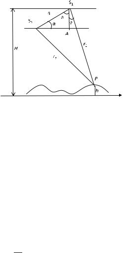
Fig. 9.5 InSAR imaging geometry: The radar signal is transmitted from antenna S1 and received simultaneously at S1 and S2. The phase difference of the two echoes is proportional to r , which depends on the baseline angle α, look angle θ , satellite altitude H , range vectors r1 and r2, and target elevation h
9.3.1.1 Basic Principle of InSAR in Elevation Measurement
InSAR in DEM generation requires that two SAR images of a target are acquired from different positions by a sensor (or sensors) with nearly the same observation angles. The phase difference between these two observations is then used to derive the elevation. The two SAR images can be taken at the same time (single-pass interferometry) or at different times (repeat-pass interferometry) over the target. Figure 9.5 depicts a simplified InSAR imaging geometry [1]. S1 and S2 are two sensor positions, r1 and r2 are range vectors from the two sensors to the target point P with elevation h, satellite altitude is H , the baseline is B, α is the baseline orientation
angle, and θ is the look angle. |
|
A complex signal returning to the SAR from the target P is expressed by |
|
S = Aej φ |
(9.7) |
where A is the amplitude and φ is the phase. Two complex SAR images (a ‘master’ and a ‘slave’) are formed from positions S1 and S2. Therefore the phase difference ψ between S1 and S2 is directly related to the path difference between r1 and r2, as follows:
ψ = − |
4π |
(9.8) |
λ r |
where λ is the SAR signal wavelength, and r = r2 − r1.
The imaging geometry in Fig. 9.5 demonstrates the relationship of B, r1, r2, α, and θ . In order to derive the formula which expresses the relationship quantitatively, two additional elements are introduced: one is point A, a perpendicular intersection point of line S1A and line S2A, and the other is angle β, the complementary angle of 90◦ to α in the right angled triangle S1S2A. According to a trigonometric theorem,
applied to the triangle S1S2P , the following equation is satisfied: |
|
|
|
||||||||||
|
r22 |
− r12 − B2 |
|
2 |
r2 |
|
B2 |
|
2r |
B cos(β |
|
θ ) |
(9.9) |
cos(β + θ ) = |
|
−2r1B |
or |
r2 = |
+ |
− |
+ |
||||||
|
1 |
|
1 |
|
|
|
|||||||
In Eq. (9.9), cos(β + θ ) can be expanded to |
|
|
|
|
|
|
|
|
|
||||
|
cos(β + θ ) = cos β cos θ − sin β sin θ |
|
|
|
(9.10) |

9 3D Digital Elevation Model Generation |
381 |
In the right angled triangle S1S2A of Fig. 9.5, sin β = cos α and cos β = sin α. Substituting these into the right-hand side of Eq. (9.10), we have
cos(β + θ ) = sin α cos θ − cos α sin θ = − sin(θ − α) |
(9.11) |
Substituting Eq. (9.11) to Eq. (9.9), the relationship of B, r1, r2, α, and θ is expressed in Eq. (9.12), and the target elevation h can be calculated from Eq. (9.13) based on the geometric relation shown in Fig. 9.5.
|
− |
|
= |
r22 |
2r1B |
2 |
|
sin(θ |
|
α) |
|
− r12 − B |
(9.12) |
||
|
= H − r1 cos θ |
|
|||||
|
|
h |
|
(9.13) |
In Eq. (9.12), r1 is replaced by r , and r2 by r + r , then it can be re-written as
sin(θ |
− |
α) |
= |
(r + r)2 − r2 − B2 |
(9.14) |
|
2rB |
||||||
|
|
|
Replacing cos θ in Eq. (9.13) by sin(θ − α) in such a way that it can be rewritten as
|
cos α 1 − |
|
sin2 |
|
− sin α sin(θ − α) |
|
h = H − r |
|
(θ − α) |
(9.15) |
In practice, the SAR altitude H , the baseline B, and the baseline orientation angle α are estimated from knowledge of the orbit, and the range r , half the roundtrip distance of radar signal, is measured by the SAR internal clock. Knowing the phase difference ψ from the interferometric fringes of two SAR images, the path difference r can be calculated from Eq. (9.8), hence sin(θ − α) can be derived from Eq. (9.14), and finally the elevation value is calculated from Eq. (9.15).
The phase difference between the two SAR images is normally represented as an interferogram, an image which is the product of the complex master image convolved with the complex slave image. It is important to appreciate that only the principal values of the phase, (i.e. modulo 2π ), can be measured from the interferogram. The 2π phase difference corresponds to one cycle of interferometric fringe. The total path difference of the two receivers is multiples of the radar wavelength, (i.e. multiples of 2π in terms of phase). The process of phase unwrapping estimates this integer number in the interferometry. It is a key process in DEM generation from InSAR.
In many cases, the InSAR imaging geometry may differ from that demonstrated in Fig. 9.5. However, the principle of deriving the target elevation from the interferogram is similar and involves the following two steps:
1.Find out the path difference from the phase difference.
2.Calculate the topography based on the path difference with other known geometric parameters.
Figure 9.5 is a simplified model and the phase of SAR signals contains other information beyond topography. For a detailed description of InSAR and a better understanding of the signal modeling, please refer to [72].