vince_j_quaternions_for_computer_graphics

Добавил:

Upload Опубликованный материал нарушает ваши авторские права? Сообщите нам.

Вуз:

Московский государственный институт электроники и математики (технический университет)

Предмет:

[НЕСОРТИРОВАННОЕ]

Файл:

Translate a point

Ttx ,ty ,tz

.pdf

Скачиваний:

118

Добавлен:

08.02.2015

Размер:

3.44 Mб

Скачать

☆

<<< < Предыдущая 1 2 3 4 5 6 7 8 910 / 1610 11 12 13 14 15 16 > Следующая >>>

76	6 3D Rotation Transforms

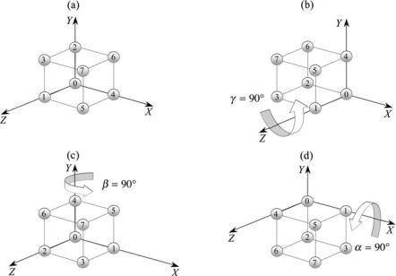
Fig. 6.3 A unit cube located at the origin

above, such rotations are called Euler rotations, and it is assumed that the reader is familiar with their construction. The triple combinations are:

Rγ ,x Rβ,y Rα,x	Rγ ,x Rβ,y Rα,z	Rγ ,x Rβ,z Rα,x	Rγ ,x Rβ,z Rα,y
Rγ ,y Rβ,x Rα,y	Rγ ,y Rβ,x Rα,z	Rγ ,y Rβ,z Rα,x	Rγ ,y Rβ,z Rα,y
Rγ ,z Rβ,x Rα,y	Rγ ,zRβ,x Rα,z	Rγ ,z Rβ,y Rα,x	Rγ ,zRβ,y Rα,z.

In order to illustrate the problem of gimbal lock we will employ a cube whose vertices are numbered 0 to 7 as shown in Fig. 6.3.

We can create a composite rotation transform by placing Rα,x , Rβ,y and Rγ ,z in any sequence—even repeating one of them twice, so long as they are separated by a different transform. As an example of the latter, we could use the sequence

Fig. 6.4 Four views of the unit cube before and during the three rotations

Rα,zRβ,y Rγ ,z

6.5 Composite Rotations

Fig. 6.5 Four views of the unit cube using the rotation sequence Rα,x Rβ,y Rγ ,z

where we rotate about the z-axis twice. However, to illustrate gimbal lock, let’s choose the sequence Rγ ,zRβ,y Rα,x and make α = β = γ = 90°, which is equivalent to rotating a point 90° about the ﬁxed x-axis, followed by a rotation of 90° about the ﬁxed y-axis, followed by a rotation of 90° about the ﬁxed z-axis. This rotation sequence is illustrated in Fig. 6.4.

Figure 6.4 (a) shows the starting position of the cube; (b) shows its position after a 90° rotation about the x-axis; (c) shows its position after a further rotation of 90° about the y-axis; and (d) the cube’s resting position after a rotation of 90° about the z-axis.

However, in spite of employing three rotations about different axes, the cube has effectively only been rotated 90° about the y-axis! The cube has been rotated twice about the axis passing through vertices 0 and 4 and once about the axis passing through vertices 0 and 1, but the axis passing through vertices 0 and 2 has been ignored. This is known as gimbal lock, and arises through an unfortunate rotation sequence combination and angles.

Reversing the composite rotation to Rα,x Rβ,y Rγ ,z does not improve matters. This composite transform is equivalent to rotating a point 90° about the ﬁxed z- axis, followed by a rotation of 90° about the ﬁxed y-axis, followed by a rotation of 90° about the ﬁxed x-axis. This rotation sequence is illustrated in Fig. 6.5.

Inspection of Fig. 6.5 (d) shows that the unit cube has been rotated 180° about the vector [1 0 1]T, i.e. an axis intersecting vertices 0 and 5. This time, the cube is rotated twice about an axis intersecting vertices 0 and 1, once about an axis intersecting vertices 0 and 4, and once again, the axis intersecting vertices 0 and 2 has

78	6 3D Rotation Transforms

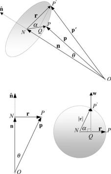
Fig. 6.6 The geometry associated with rotating a point about an arbitrary axis

been ignored. It is not difﬁcult to see why Euler rotations cause so many problems. So let’s continue and see how we can rotate about an arbitrary axis.

6.6 Rotating About an Arbitrary Axis

There is nothing fundamentally wrong with individual Euler transforms—it is the way they are combined to effect a rotation that is ﬂawed. Ideally, we require a rotation transform that permits us to specify the axis and angle of rotation, which is what we will compute. The ﬁrst technique uses matrices and trigonometry and is rather laborious. The second approach employs vector analysis and is quite succinct.

6.6.1 Matrices

We begin by deﬁning an axis using a unit vector nˆ about which a point P is rotated α to P as shown in Fig. 6.6. And as we only have access to matrices that rotate points about the Cartesian axes, this unit vector has to be temporarily aligned with a Cartesian axis. In the following example we choose the x-axis. During the alignment process, the point P is subjected to the transforms necessary to align the unit vector with the x-axis. We then rotate P , α about the x-axis. To complete the operation, the rotated point is subjected to the transforms that return the unit vector to its original position.

Although matrices provide a powerful tool for undertaking this sort of work, it is, nevertheless, extremely tedious, but a good exercise for improving one’s algebraic skills!

Figure 6.6 shows a point P (x, y, z) to be rotated through an angle α to P (x , y , z ) about an axis deﬁned by

nˆ = ai + bj + ck.

6.6 Rotating About an Arbitrary Axis

The transforms to achieve this operation is expressed as follows:

x						x
y		R	−	φ,y Rθ ,zRα,x R	θ ,z Rφ,y	y
z	=		−	−		z

which aligns the axis of rotation with the x-axis, performs the rotation of P through an angle α about the x-axis, and returns the axis of rotation back to its original position. Therefore,

Rφ,y

R θ ,z

sin θ

cos θ

cos φ

sin φ

cos θ

sin

Rα,x

= − sin φ

cos φ

− = −

cos α

− sin α

Rθ ,z

sin θ

cos θ

cos

− sin θ

R φ,y

sin α

cos α

−

cos φ

sin φ

−

= sin φ

cos φ

Let

R φ,y Rθ ,zRα,x R θ ,zRφ,y

a21

a22

a23

a11

a12

a13

−

= a31

a32

a33

where by multiplying the matrices together we ﬁnd that:

a11 = cos2 φ cos2 θ + cos2 φ sin2 θ cos α + sin2 φ cos α

a12 = cos φ cos θ sin θ − cos φ sin θ cos θ cos α − sin φ cos θ sin α a13 = cos φ sin φ cos2 θ + cos φ sin φ sin2 θ cos α + sin2 φ sin θ sin α

+ cos2 φ sin θ sin α − cos φ sin φ cos α

a21 = sin θ cos θ cos φ − cos θ sin θ cos φ cos α + cos θ sin φ sin α a22 = sin2 θ + cos2 θ cos α

a23 = sin θ cos θ sin φ − cos θ sin θ sin φ cos α − cos θ cos φ sin α a31 = cos φ sin φ cos2 θ + cos φ sin φ sin2 θ cos α − cos2 φ sin θ sin α

= − cos φ sin φ cos α

a32 = sin φ cos θ sin θ − sin φ sin θ cos θ cos α + cos φ cos θ sin α a33 = sin2 φ cos2 θ + sin2 φ sin2 θ cos α − cos φ sin φ sin θ sin α

+ cos φ sin φ sin θ sin α + cos2 φ cos α.

After much trigonometric substitution we arrive at the transform

	y			K + cos α		2	K	−	cos α
	y		abK		c sin α	b	K		cos α
	xp		a2			abK			c sin α
zp		=	acK		+ b sin α	bcK		+a sin α
	p				−			+

bcK	+ a sin α	yp
acK	b sin α	xp
	−	zp
c2K + cos α		zp

80	6 3D Rotation Transforms

Fig. 6.7 A view of the geometry associated with rotating a point about an arbitrary axis

Fig. 6.8 A cross-section and plan view of the geometry associated with rotating a point about an arbitrary axis

where

K = 1 − cos α.

6.6.2 Vectors

Now let’s solve the same problem using vectors. Figure 6.7 shows a view of the geometry associated with the task at hand. For clariﬁcation, Fig. 6.8 shows a crosssection and a plan view of the geometry.

The axis of rotation is given by the unit vector

nˆ = ai + bj + ck.

P (xp , yp zp ) is the point to be rotated by angle α to P (xp , yp , zp ).
O is the origin, whilst p and p are position vectors for P and P respectively.
From Figs. 6.7 and 6.8:	ON	N Q	−−→
p
=	−−→	+ −−→ +		.
			QP

−−→

To ﬁnd ON :

|n| = |p| cos θ = nˆ · p

6.6 Rotating About an Arbitrary Axis

therefore,

−−→

n n

−−→

= ˆ

(

ˆ ·

To ﬁnd

N Q:

= N P

−−→ =

N P

N Q

cos αr

but

therefore,

p = n + r = nˆ (nˆ · p) + r

and

r = p − nˆ (nˆ · p)

−−→

−

ˆ ˆ

−−→

N Q

n(n

p) cos α.

To ﬁnd

Let

where

nˆ × p = w

but

|w| = |nˆ | · |p| sin θ = |p| sin θ

therefore,

|r| = |p| sin θ

Now

|w| = |r|.

= sin α

N P

|r|

|w|

therefore,

−−→

QP = w sin α = (nˆ × p) sin α

then

p = nˆ (nˆ · p) + p − nˆ (nˆ · p) cos α + (nˆ × p) sin α

and

p = p cos α + nˆ (nˆ · p)(1 − cos α) + (nˆ × p) sin α.

Let

K = 1 − cos α

82	6 3D Rotation Transforms

Fig. 6.9 Rotating the point

P through 180° to P

then

p = p cos α + nˆ (nˆ · p)K + (nˆ × p) sin α

and

p = (xp i + yp j + zp k) cos α + (ai + bj + ck)(axp + byp + czp )K

+(bzp − cyp )i + (cxp − azp )j + (ayp − bxp )k sin α p = xp cos α + a(axp + byp + czp )K + (bzp − cyp ) sin α i

+yp cos α + b(axp + byp + czp )K + (cxp − azp ) sin α j

+zp cos α + c(axp + byp + czp )K + (ayp − bxp ) sin α k

p = xp a2K + cos α + yp (abK − c sin α) + zp (acK + b sin α) i

+xp (abK + c sin α) + yp b2K + cos α + zp (bcK − a sin α) j

+xp (acK − b sin α) + yp (bcK + a sin α) + zp c2K + cos α k

which unpacks into the transform:

	y		a K + cos α		2	K	−	cos α
	y		abK	c sin α	b	K		cos α
	xp	=	2		abK			c sin α
zp		=	acK	+ b sin α	bcK		+a sin α
	p			−			+

where

K = 1 − cos α

bcK	+ a sin α	yp
acK	b sin α	xp
	−	zp
c2K + cos α		zp

and is identical to the transform derived using matrices.

Let’s test the transform with a simple example that can be easily√ veriﬁed.√If we rotate the point P (10, 0, 0), 180° about an axis deﬁned by nˆ = (1/ 2)i + (1/ 2)k, it should be rotated to P (0, 0, 10) as shown in Fig. 6.9. Therefore,

α = 180°, cos α = −1,				sin α = 0, K = 2,
1				1
a =	√	, b	= 0,	c =	√
2				2

6.7 Summary				83
and	0 −1		0	0
0	0 −1		0	0
0	0	0	1	10
10 = 1		0	0 0

which conﬁrms our prediction.

6.7 Summary

In this chapter we have reviewed the matrix rotation transforms for rotating a point about one of the three Cartesian axes. By employing homogeneous coordinates, the translation transform can be integrated to rotate points about an off-set axis parallel with one of the Cartesian axes.

Composite rotations are created by combining the matrices representing the individual rotations about three successive axes. Such rotations are known as Euler rotations, and there are twelve ways of combining these matrices. Unfortunately, one of the problems with such transforms is that they suffer from gimbal lock, where one degree of freedom is lost under certain angle combinations. Another problem, is that it is difﬁcult to predict how a point moves in space when animated by a composite transform, although they are widely used for positioning objects in world space.

Finally, matrices and vectors were used to develop a transform for rotating a point about an arbitrary axis.

6.7.1 Summary of Transforms

Rotate a point about the x-, y-, z-axes					− sin β
Rβ,x		0	cos β		− sin β
	=	1	0			0
Rβ,y	=	0	sin β			cos β
Rβ,y			0		1	0
		cos β			0	sin β
Rβ,z	= − sin β				0	cos β
Rβ,z	sin β			cos β			0
	=	cos β		− sin β			0
	=		0		0		1

3D Rotation Transforms

Rotate a point about off-set x-, y-, z-axes

tz sin β

Rβ,x,(0,t

,t )

cos β

− sin β

ty (1

cos β)

sin β

cos β

tz(1

− cos β)

+ ty sin β

−

sin β

cos β

sin β

cos β)

Rβ,y,(tx ,0,tz )

−

sin β

cos β

tz(1

−

cos β)

tx sin β

sin β

cos β

− cos β)

+ tx sin β

Rβ,z,(tx ,ty ,0)

cos β

− sin β

−

cos β)

−

ty sin β

Rotate a point about an arbitrary axis

a2K

cos α

abK

c sin α

acK

b sin α

abK

+c sin α

b2K

− cos α

bcK + a sin α

α,nˆ =

−

acK − b sin α

bcK + a sin α

c2K + cos α

K = 1 − cos α

nˆ = ai + bj + ck.

6.8 Worked Examples

Here are some further worked examples that employ the ideas described above. In some cases, a test is included to conﬁrm the result.

Example 1 Develop a rotation transform to rotate a point about an axis off-set to the y-axis.

Let the off-set axis intersect the point (tx , 0, tz). Therefore, the homogeneous transform for this rotation is

x		x
y	= Ttx ,0,tz Rβ,y T−tx ,0,−tz	y
z	= Ttx ,0,tz Rβ,y T−tx ,0,−tz	z
1		1

where

T−tx ,0,−tz creates a temporary origin

Rβ,y	rotates β about the temporary y-axis
Ttx ,0,tz	returns to the original position
and

6.8 Worked Examples

									1			0		0	tx
				Ttx					0			1		0	0
				Ttx	,0,tz	=			0		0 1 tz
									0			0		0	1

									1			0		0	−tx
			T−tx ,0,−tz						0			1		0	0
			T−tx ,0,−tz			=			0		0 1 −tz
									0			0		0	1

										cos β					0	sin β		0
				Rβ,y							0				1		0	0
				Rβ,y		=			−		sin β				0	cos β		0	.
									−		0				0		0	1
Therefore,
Therefore,
Ttx ,0,tz Rβ,y T−tx ,0,−tz																						−tx
	1	0	0	tx			cos β					0			sin β		0		1	0	0	−tx
=	0	1	0	0				0				1			0		0		0 1 0			0
=	0	0	1	tz			− sin β					0			cos β		0		0	0	1	−tz
	0	0	0	1				0				0			0		1		0 0 0			1

	1	0	0	tx			cos β					0			sin β		−	tx cos β			tz sin β
=	0	1	0	0				0				1			0		−		0−
=	0	0	1	tz			−	sin β				0			cos β		tx sin β − tz cos β
	0	0	0	1			−	0				0			0				1

	cos β			0	sin β			t							β)		t sin β
=		0		1	0					x (1		− cos 0				− z
=	−	sin β		0	cos β			tz (1				−	cos β)			+	tx sin β		.
	−	0		0	0							−			1	+

Example 2 Compute the rotation transform for Rγ ,x Rβ,y Rα,x																				and see if it suffers

from gimbal lock when α = β = γ = 90°. What is the axis and angle of rotation? Using the notation cβ = cos β and sβ = sin β , the composite transform is

Rγ ,x Rβ,y Rα,x		0	cγ	−sγ		0	1	0	0	cα	−sα
		1	0	0		cβ	0	sβ	1	0	0
	= 0		sγ	cγ	−sβ		0	cβ 0		sα	cα

	sγ sβ			(cγ cα		β sγ cβ sα ) ( cγ sα			sγ cβ cα )
			cβ			s sα	sβ cα
	= −cγ sβ					−	−	−
R90°,x R90°,y R90°,x	= −cγ sβ			(sγ cα + cγ cβ sα ) (−sγ sα + cγ cβ cα )
R90°,x R90°,y R90°,x		1	0	0	.
	=	0	1	0
	=	0	0	−1

Figure 6.10 shows a cube at each stage of rotation, and it is clear that gimbal lock is not present as the cube is rotated through each of its orthogonal axes. The axis

<<< < Предыдущая 1 2 3 4 5 6 7 8 910 / 1610 11 12 13 14 15 16 > Следующая >>>

Соседние файлы в предмете [НЕСОРТИРОВАННОЕ]

#
23.11.2019146.94 Кб6training.doc
#
08.02.2015491.01 Кб6Uchebnoe_posobie_GMBSS_VFPS.doc
#
08.02.20151.53 Mб3UNIVER_30_08.pdf
#
04.08.2019212.48 Кб2var_test._zadanii-1.doc
#
20.04.2019215.04 Кб1var_test._zadanii-2.doc
#
08.02.20153.44 Mб118vince_j_quaternions_for_computer_graphics.pdf
#
21.11.20193.06 Mб2workbook-infcs-labs.doc
#
08.02.2015264.7 Кб5zachet_ekonom (1).doc
#
08.02.2015418.97 Кб10_Лр_2012.pdf
#
08.02.2015294.4 Кб9Алгоритмизация вычислений НИУ ВШЭпрогр 2014_15.doc
#
08.02.2015211.45 Кб16Архитектура ЭВМ - испр.docx