vince_j_quaternions_for_computer_graphics

Fig. 6.10 Four views of the unit cube before and during the three rotations R90°,x R90°,y R90°,x

of rotation is through the vertices 0 and 6, i.e. [1 1 0]T and the angle of rotation is 180°.

Example 3 Show that the rotation matrix for rotating points about an arbitrary axis works for the three Cartesian axes.

Starting with the matrix:

nˆ = ai + bj + ck.

Rotating about the x-axis:

nˆ = ai

therefore, a = 1 and b = c = 0:

Rotating about the y-axis:

nˆ = bj

which confirms that any point rotated twice by the rotation matrix returns to its original point.

Fig. 7.1 Rodrigues’ spherical triangle showing l, m and n

7.2 Some History

Benjamin Olinde Rodrigues (1795–1851) was born in Bordeaux, France. He studied in Paris, and in 1816 was awarded his doctorate at the age of 21. The subject of his thesis was solving Legendre polynomials, and Rodrigues proposed a solution which is still known as the Rodrigues formula.

Although he pursued a career in politics and banking, his doctoral research confirms that he was more than just a ‘recreational’ mathematician, for in 1840 he published a mathematical paper in the Annales de Mathématiques Pures et Appliquées on transformation groups [20]. The paper contains a formula describing a geometric construction equating two successive rotations about different axes, with a third rotation about another axis. Today, we know this correspondence as the Euler-Rodrigues Parameterisation. Euler had already shown in 1775 that a single rotation could represent two successive rotations about different axes, but did not provide an algebraic solution.

If we represent a rotation α about an axial vector a as Rα,a, then Rodrigues provided a solution to

Rodrigues did not use the vector notation employed in (7.1) and (7.2), as this was yet to be defined by Hamilton, but he did employ the algebraic equivalent of these vector products. Figure 7.1 shows the spherical triangle formed by the axes and angles of rotation used by Rodrigues.

Equations (7.1) and (7.2) contain some features familiar to the quaternion product, which become obvious with the following analysis. We start by defining the quaternions

where (7.3) and (7.4) are identical to (7.1) and (7.2) respectively. Although Rodrigues had not invented quaternions in the form of

q = s + ai + bj + ck,

he had discovered the coefficients of a quaternion product before Hamilton. C’est la vie!

Hamilton invented quaternions in October 1843, and by December of the same year, his friend, Irish mathematician, John Thomas Graves (1806–1870), had invented octaves, which would eventually be called octonions. The British mathematician, Arthur Cayley (1821–1895), had also been intrigued by Hamilton’s quaternions, and independently invented octonions in 1845. Octonions eventually became known as Cayley numbers rather than octaves, simply because Graves did not publish his results until 1848—three years after Cayley!

Just as quaternions can be defined in terms of ordered pairs of complex numbers, the octaves, or octonions, can be defined as ordered pairs of quaternions.

7.2.1 Composition Algebras

When a specific law forms the basis of an algebra, it is called a composition algebra. For example, we know that in ordinary arithmetic

a2b2 = (ab)2 a, b R

e.g.

3242 = 122

where a square law is the composition law.

We discovered in Chap. 4 that for two complex numbers:

|z1||z2| = |z1z2| z1, z2 C |z1|2|z2|2 = |z1z2|2.

For example, given

z1 = a1 + b1i z2 = a2 + b2i

then

a12 + b12 a22 + b22 = (a1a2 − b1b2)2 + (a1b2 + a2b1)2

which is a two-square law.

In Chap. 5 we noted that for two quaternions:

|qa |2|qb |2 = |qa qb |2 qa , qb H.

For example, given

qa = [sa , xa i + ya j + za k] qb = [sb , xb i + yb j + zb k]

then

sa2 + xa2 + ya2 + za2 sb2 + xb2 + yb2 + zb2 = (sa sb − xa xb − ya yb − za zb )2

+ (sa xb + sb xa + ya zb − yb za )2 + (sa yb + sb ya + za xb − zb xa )2 + (sa zb + sb za + xa yb − xb ya )2

which is a four-square law.

In addition to complex numbers, quaternions occupy a central place in mathematical systems, and today there are four such composition algebras: real R, complex C, quaternion H, and octonion O that obey an n-square identity used to compute their norms. In 1898 the German mathematician, Adolf Hurwitz (1859–1919), proved that the product of the sum of n squares by the sum of n squares is the sum of n squares only when n is equal to 1, 2, 4 and 8, which are represented by the reals, complex numbers, quaternions and octonions. This is known as ‘Hurwitz’s Theorem’ or the ‘1, 2, 4, 8 Theorem’. No other system is possible, which shows how important quaternions are within the realm of mathematics. Consequently, Hamilton’s search for a system of triples was futile, because there is no three-square identity.

Now let’s investigate how quaternions are used to rotate vectors about an arbitrary axis.

7.3 Quaternion Products

A quaternion q is the union of a scalar s and a vector v: q = [s, v] s R, v R3.

If we express v in terms of its components, we have

q = [s, xi + yj + zk] s, x, y, z R.

Hamilton had hoped that a quaternion could be used like a complex rotor, where we saw in Chap. 2 that

Rθ = cos θ + i sin θ

rotates a complex number by θ . Could a unit-norm quaternion q be used to rotate a vector stored as a pure quaternion p? Well yes, but only in a restricted sense. To understand this, let’s construct the product of a unit-norm quaternion q and a pure quaternion p. The unit-norm quaternion q is defined as

|vˆ | = 1 s2 + λ2 = 1

and the pure quaternion p stores the vector p to be rotated:

p = [0, p] p R3.

Let’s compute the product p = qp and examine the vector part of p to see if p is rotated:

We can see from (7.6) that the result is a general quaternion with a scalar and a vector component.

7.3.1 Special Case

The ‘restricted sense’ referred to above is that vˆ must be perpendicular to p, which makes the dot product term −λvˆ · p in (7.6) vanish, and we are left with the pure quaternion

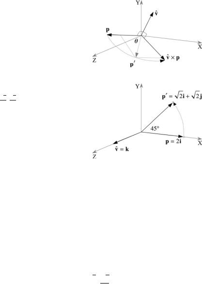
Figure 7.2 illustrates this scenario, where p is perpendicular to vˆ , and vˆ × p is perpendicular to the plane containing p and vˆ . Now because vˆ is a unit vector,

Fig. 7.2 Three orthogonal vectors p, vˆ and vˆ × p

Fig. 7.3 The vector 2i is

rotated 45° by the quaternion

√ √

q = [ 22 ,

|p| = |vˆ × p|, which means that we have two orthogonal vectors, i.e. p and vˆ × p, with the same length. Therefore, to rotate p about vˆ , all that we have to do is make s = cos θ and λ = sin θ in (7.7):

p = [0, p ]

= [0, cos θ p + sin θ vˆ × p].

For example, to rotate a vector about the z-axis, q ’s vector vˆ must be aligned with the z-axis as shown in Fig. 7.3. If we make the angle of rotation θ = 45° then

q= [s, λvˆ ]

=[cos θ , sin θ k]

√√

and if the vector to be rotated is p = 2i, then

p= [0, p] = [0, 2i].

There are now four product combinations worth exploring: qp, pq , q−1p and pq−1. It’s not worth considering qp−1 and p−1q as p−1 simply reverses the direction of p.

is the angle of rotation, then

qp = pq−1 pq = q−1p.